基于Keras的深度学习的相关基础概念的讲解
2018-03-08 14:42
696 查看
深度学习
目录1.softmax
2.损失函数
3.激活函数
4.sigmoid
5.ReLu
6.学习速率
7.Dropout
一、基础篇
神经网络中的每个神经元 对其所有的输入进行加权求和,并添加一个被称为偏置(bias) 的常数,然后通过一些非线性激活函数来反馈结果。1. softmax
softmax主要用来做多分类问题,是logistic回归模型在多分类问题上的推广,softmax 公式: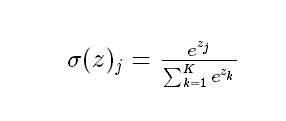
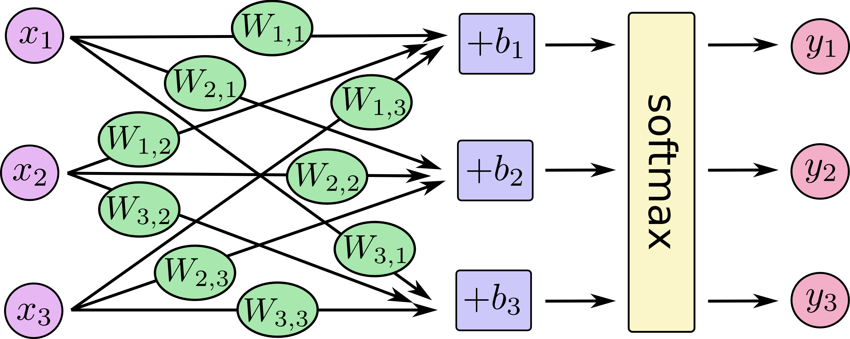
当k=2时,转换为逻辑回归形式。softmax一般作为神经网络最后一层,作为输出层进行多分类,Softmax的输出的每个值都是>=0,并且其总和为1,所以可以认为其为概率分布。softmax 示意图
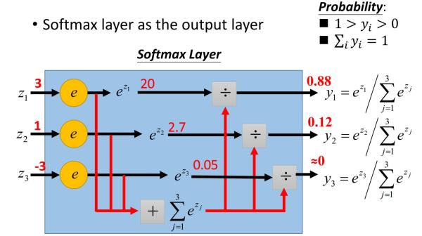
softmax 输出层示意图
In [1]:
%pylab inline
Populating the interactive namespace from numpy and matplotlibIn [2]:
from IPython.display import SVG
from keras.datasets import mnist
from keras.models import Sequential
from keras.layers import Dense, Dropout, Activation, Reshape
from keras.optimizers import SGD, Adam
from keras.utils.visualize_util import model_to_dot
from keras.utils import np_utils
import matplotlib.pyplot as plt
import tensorflow as tf
import pandas as pd
Using TensorFlow backend.In [3]:
#设置随机数种子,保证实验可重复
import numpy as np
np.random.seed(0)
#设置线程
THREADS_NUM = 20
tf.ConfigProto(intra_op_parallelism_threads=THREADS_NUM)

(X_train, Y_train),(X_test, Y_test) = mnist.load_data()
print('原数据结构:')
print(X_train.shape, Y_train.shape)
print(X_test.shape, Y_test.shape)

#数据变换
#分为10个类别
nb_classes = 10

x_train_1 = X_train.reshape(60000, 784)
#x_train_1 /= 255
#x_train_1 = x_train_1.astype('float32')
y_train_1 = np_utils.to_categorical(Y_train, nb_classes)
print('变换后的数据结构:')
print(x_train_1.shape, y_train_1.shape)

x_test_1 = X_test.reshape(10000, 784)
y_test_1 = np_utils.to_categorical(Y_test, nb_classes)
print(x_test_1.shape, y_test_1.shape)
原数据结构: ((60000, 28, 28), (60000,)) ((10000, 28, 28), (10000,)) 变换后的数据结构: ((60000, 784), (60000, 10)) ((10000, 784), (10000, 10))In [5]:
# 构建一个softmax模型
# neural network with 1 layer of 10 softmax neurons
#
# · · · · · · · · · ·       (input data, flattened pixels)       X [batch, 784]        # 784 = 28 * 28
# \x/x\x/x\x/x\x/x\x/    -- fully connected layer (softmax)      W [784, 10]     b[10]
#   · · · · · · · ·                                              Y [batch, 10]

# The model is:
#
# Y = softmax( X * W + b)
#              X: matrix for 100 grayscale images of 28x28 pixels, flattened (there are 100 images in a mini-batch)
#              W: weight matrix with 784 lines and 10 columns
#              b: bias vector with 10 dimensions
#              +: add with broadcasting: adds the vector to each line of the matrix (numpy)
#              softmax(matrix) applies softmax on each line
#              softmax(line) applies an exp to each value then divides by the norm of the resulting line
#              Y: output matrix with 100 lines and 10 columns

model = Sequential()
model.add(Dense(nb_classes, input_shape=(784,)))#全连接,输入784维度, 输出10维度,需要和输入输出对应
model.add(Activation('softmax'))

sgd = SGD(lr=0.005)
#binary_crossentropy,就是交叉熵函数
model.compile(loss='binary_crossentropy',
optimizer=sgd,
metrics=['accuracy'])

#model 概要
model.summary()
____________________________________________________________________________________________________ Layer (type) Output Shape Param # Connected to ==================================================================================================== dense_1 (Dense) (None, 10) 7850 dense_input_1[0][0] ____________________________________________________________________________________________________ activation_1 (Activation) (None, 10) 0 dense_1[0][0] ==================================================================================================== Total params: 7,850 Trainable params: 7,850 Non-trainable params: 0 ____________________________________________________________________________________________________In [6]:
SVG(model_to_dot(model).create(prog='dot', format='svg'))Out[6]:dense_input_1: InputLayerdense_1: Denseactivation_1: ActivationIn [4]:
from keras.callbacks import Callback, TensorBoard
import tensorflow as tf

#构建一个记录的loss的回调函数
class LossHistory(Callback):
def on_train_begin(self, logs={}):
self.losses = []

def on_batch_end(self, batch, logs={}):
self.losses.append(logs.get('loss'))

# 构建一个自定义的TensorBoard类,专门用来记录batch中的数据变化
class BatchTensorBoard(TensorBoard):
def __init__(self,log_dir='./logs',
histogram_freq=0,
write_graph=True,
write_images=False):
super(BatchTensorBoard, self).__init__()
self.log_dir = log_dir
self.histogram_freq = histogram_freq
self.merged = None
self.write_graph = write_graph
self.write_images = write_images
self.batch = 0
self.batch_queue = set()

def on_epoch_end(self, epoch, logs=None):
pass

def on_batch_end(self,batch,logs=None):
logs = logs or {}

self.batch = self.batch + 1

for name, value in logs.items():
if name in ['batch', 'size']:
continue
summary = tf.Summary()
summary_value = summary.value.add()
summary_value.simple_value = float(value)
summary_value.tag = "batch_" + name
if (name,self.batch) in self.batch_queue:
continue
self.writer.add_summary(summary, self.batch)
self.batch_queue.add((name,self.batch))
self.writer.flush()
In [54]:tensorboard = TensorBoard(log_dir='/home/tensorflow/log/softmax/epoch') my_tensorboard = BatchTensorBoard(log_dir='/home/tensorflow/log/softmax/batch') model.fit(x_train_1, y_train_1, nb_epoch=20, verbose=0, batch_size=100, callbacks=[tensorboard, my_tensorboard])Out[54]:
<keras.callbacks.History at 0xa86d650>
损失函数
损失函数(loss function),是指一种将一个事件(在一个样本空间中的一个元素)映射到一个表达与其事件相关的经济成本或机会成本的实数上的一种函数,在统计学中损失函数是一种衡量损失和错误(这种损失与“错误地”估计有关,如费用或者设备的损失)程度的函数。交叉熵(cross-entropy)就是神经网络中常用的损失函数。交叉熵性质:(1)非负性。(2)当真实输出a与期望输出y接近的时候,代价函数接近于0.(比如y=0,a~0;y=1,a~1时,代价函数都接近0)。
一个比较简单的理解就是使得 预测值Yi和真实值Y' 对接近,即两者的乘积越大,coss-entropy越小。交叉熵和准确度变化图像可以看 TensorBoard 。
梯度下降
如果对于所有的权重和所有的偏置计算交叉熵的偏导数,就得到一个对于给定图像、标签和当前权重和偏置的「梯度」,如图所示: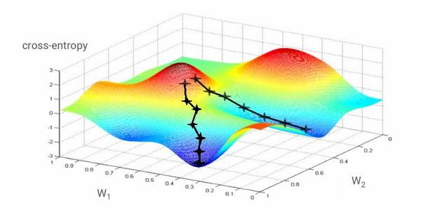
我们希望损失函数最小,也就是需要到达交叉熵最小的凹点的低部。在上图中,交叉熵被表示为一个具有两个权重的函数。而学习速率,即在梯度下降中的步伐大小。In [72]:
#模型的测试误差指标
print(model.metrics_names)
# 对测试数据进行测试
model.evaluate(x_test_1, y_test_1,
verbose=1,
batch_size=100)
['loss', 'acc']
9800/10000 [============================>.] - ETA: 0s
Out[72]:
[0.87580669939517974, 0.94387999653816224]上面,我们探索了softmax对多分类的支持和理解,知道softmax可以作为一个输出成层进行多分类任务。但是,这种分类任务解决的都是线性因素形成的问题,对于非线性的,特别是异或问题,如何解决呢?这时,一种包含多层隐含层的深度神经网络的概念被提出。
3. 激活函数
激活函数(activation function)可以使得模型加入非线性因素的。解决非线性问题有两个办法:线性变换、引入非线性函数。(1)线性变换(linear transformation)原本一个线性不可分的模型如:X^2 + Y^2 = 1其图形如下图所示:In [21]:fig = plt.figure(0) degree = np.random.rand(50)*np.pi*2 x_1 = np.cos(degree)*np.random.rand(50) y_1 = np.sin(degree)*np.random.rand(50) x_2 = np.cos(degree)*(1+np.random.rand(50)) y_2 = np.sin(degree)*(1+np.random.rand(50)) # x_3 和 y_3 就是切分线 t = np.linspace(0,np.pi*2,50) x_3 = np.cos(t) y_3 = np.sin(t) scatter(x_1,y_1,c='red',s=50,alpha=0.4,marker='o') scatter(x_2,y_2,c='black',s=50,alpha=0.4,marker='o') plot(x_3,y_3)Out[21]:
[<matplotlib.lines.Line2D at 0x86c7510>]将坐标轴进行高维变换,横坐标变成X^2,纵坐标变成 Y^2,这是表达式变为了 X + Y = 1,这样,原来的非线性问题,就变成了一个线性可分的问题,变成了一个简单的一元一次方程了。详细可以参见下图:In [31]:
fig2 = plt.figure(1)
#令新的横坐标变成x^2,纵坐标变成 Y^2
x_4 = x_1**2
y_4 = y_1**2
x_5 = x_2**2
y_5 = y_2**2

# 这样就可以构建一个一元线性方程进行拟合
x_6 = np.linspace(-1,2,50)
y_6 = 1 - x_6

scatter(x_4,y_4,c='red',s=50,alpha=0.4,marker='o')
scatter(x_5,y_5,c='black',s=50,alpha=0.4,marker='o')
plot(x_6,y_6)
Out[31]:
[<matplotlib.lines.Line2D at 0x984bf10>](2)引入非线性函数异或是一种基于二进制的位运算,用符号XOR 表示(Python中的异或操作符为 ^ ),其运算法则是对运算符两侧数的每一个二进制位,同值取0,异值取1。下面是一个典型的异或表:In [37]:
table = {'x':[1,0,1,0],'y':[1,0,0,1]}
df = pd.DataFrame(table)
df['z'] = df['x']^df['y']
dfOut[37]:| x | y | z | |
|---|---|---|---|
| 0 | 1 | 1 | 0 |
| 1 | 0 | 0 | 0 |
| 2 | 1 | 0 | 1 |
| 3 | 0 | 1 | 1 |
fig3 = plt.figure(2)
groups = df.groupby('z')
for name, group in groups:
scatter(group['x'],group['y'],label=name,s=50,marker='o')
那么如果可以构建一个函数拟合这样的图形呢?即如何构建一个f(),使得:f(x,y)=z呢?为了解决问题,我们来构建一个两层的神经网络,该神经网络有两个激活函数,F(x,y)和 H(x,y), 具体如下图所示:
F(x,y)为一个阈值为1的阈值函数:即:当AX+BY>1时候,F(x,y) = 1;否则为0;
if AX+BY > 1:
F = 1
else:
F = 0
H(x,y)为一个阈值为0的阈值函数:
if AX+BY > 0:
H = 1
else:
H = 0
图中线的数字表示权重值,
- 对于(1,1)的点,第二层从左到右隐藏层的值分别为(1,1,1),最后输出为(1,1,1)*(1,-2,1)=0;

- 对于(0,0)的点,第二层从左到右隐藏层的值分别为(0,0,0),最后输出为(0,0,0)*(1,-2,1)=0;

- 对于(1,0)的点,第二层从左到右隐藏层的值分别为(1,0,0),最后输出为(1,0,0)*(1,-2,1)= 1;

- 对于(0,1)的点,第二层从左到右隐藏层的值分别为(0,0,1),最后输出为(0,0,1)*(1,-2,1)= 1;
In [67]:
first_hidder_layer_table = {'x':[1,0,1,0],'y':[1,0,0,0],'z':[1,0,0,1],'output':[0,0,1,1]}
first_hidder_layer_data = pd.DataFrame(first_hidder_layer_table)
first_hidder_layer_dataOut[67]:| output | x | y | z | |
|---|---|---|---|---|
| 0 | 0 | 1 | 1 | 1 |
| 1 | 0 | 0 | 0 | 0 |
| 2 | 1 | 1 | 0 | 0 |
| 3 | 1 | 0 | 0 | 1 |
from mpl_toolkits.mplot3d import Axes3D
fig4 = plt.figure(3)
ax = fig4.add_subplot(111, projection='3d')
groups = first_hidder_layer_data.groupby('output')
for name, group in groups:
ax.scatter(group['x'],group['y'],group['z'],label=name,c=np.random.choice(['black','blue']),s=50,marker='o')
ax.set_xlabel('X Label')
ax.set_ylabel('Y Label')
ax.set_zlabel('Z Label')Out[74]:<matplotlib.text.Text at 0xb7b0d90>经过变换后的数据是线性可分的(n维,比如本例中可以用平面将两个不同颜色的点切分)更多的操作可以参考tensorflow提供的一个神经网络的网页小程序,通过自己调整程序参数可以更深刻理解神经网络、激活函数的作用。演示网址:http://playground.tensorflow.org/可以自己建立一个小型神经网络帮助理解。
4. sigmoid
sigmoid是一个用来做二分类的"S"形逻辑回归曲线sigmoid公式:
sigmoid图像:

其抑制两头,对中间细微变化敏感,因此sigmoid函数作为最简单常用的神经网络激活层被使用。优点:(1)输出范围(0,1),数据在传递的过程中不容易发散(2)单向递增(3)易求导sigmod有个缺点,sigmoid函数反向传播时,很容易就会出现梯度消失,在接近饱和区的时候,导数趋向0,会变得非常缓慢。因此,在优化器选择时选用Adam优化器。Adam 也是基于梯度下降的方法,但是每次迭代参数的学习步长都有一个确定的范围,不会因为很大的梯度导致很大的学习步长,参数的值比较稳定。有利于降低模型收敛到局部最优的风险,而SGD容易收敛到局部最优,如果下面代码中的optimizer改成SGD的化,在一次epoch后就acc值不会改变了,陷入局部最优In [46]:
# 构建一个五层sigmod全连接神经网络
# neural network with 5 layers
#
# · · · · · · · · · ·       (input data, flattened pixels)       X [batch, 784]   # 784 = 28*28
# \x/x\x/x\x/x\x/x\x/    -- fully connected layer (sigmoid)      W1 [784, 200]      B1[200]
#  · · · · · · · · ·                                             Y1 [batch, 200]
#   \x/x\x/x\x/x\x/      -- fully connected layer (sigmoid)      W2 [200, 100]      B2[100]
#    · · · · · · ·                                               Y2 [batch, 100]
#    \x/x\x/x\x/         -- fully connected layer (sigmoid)      W3 [100, 60]       B3[60]
#     · · · · ·                                                  Y3 [batch, 60]
#     \x/x\x/            -- fully connected layer (sigmoid)      W4 [60, 30]        B4[30]
#      · · ·                                                     Y4 [batch, 30]
#      \x/               -- fully connected layer (softmax)      W5 [30, 10]        B5[10]
#       ·                                                        Y5 [batch, 10]

model = Sequential()
model.add(Dense(200, input_shape=(784,)))#全连接,输入784维度, 输出10维度,需要和输入输出对应
model.add(Activation('sigmoid'))
model.add(Dense(100))# 除了首层需要设置输入维度,其他层只需要输入输出维度就可以了,输入维度自动继承上层。
model.add(Activation('sigmoid'))
model.add(Dense(60))
model.add(Activation('sigmoid'))
model.add(Dense(30))            #model.add(Activation('sigmoid'))和model.add(Dense(30))可以合并写出
model.add(Activation('sigmoid'))#model.add(Dense(30,activation='softmax'))
model.add(Dense(10))
model.add(Activation('softmax'))

sgd = Adam(lr=0.003)
model.compile(loss='binary_crossentropy',
optimizer=sgd,
metrics=['accuracy'])

#model 概要
model.summary()
____________________________________________________________________________________________________ Layer (type) Output Shape Param # Connected to ==================================================================================================== dense_23 (Dense) (None, 200) 157000 dense_input_7[0][0] ____________________________________________________________________________________________________ activation_23 (Activation) (None, 200) 0 dense_23[0][0] ____________________________________________________________________________________________________ dense_24 (Dense) (None, 100) 20100 activation_23[0][0] ____________________________________________________________________________________________________ activation_24 (Activation) (None, 100) 0 dense_24[0][0] ____________________________________________________________________________________________________ dense_25 (Dense) (None, 60) 6060 activation_24[0][0] ____________________________________________________________________________________________________ activation_25 (Activation) (None, 60) 0 dense_25[0][0] ____________________________________________________________________________________________________ dense_26 (Dense) (None, 30) 1830 activation_25[0][0] ____________________________________________________________________________________________________ activation_26 (Activation) (None, 30) 0 dense_26[0][0] ____________________________________________________________________________________________________ dense_27 (Dense) (None, 10) 310 activation_26[0][0] ____________________________________________________________________________________________________ activation_27 (Activation) (None, 10) 0 dense_27[0][0] ==================================================================================================== Total params: 185,300 Trainable params: 185,300 Non-trainable params: 0 ____________________________________________________________________________________________________In [77]:
SVG(model_to_dot(model).create(prog='dot', format='svg'))Out[77]:dense_input_11: InputLayerdense_23: Denseactivation_23: Activationdense_24: Denseactivation_24: Activationdense_25: Denseactivation_25: Activationdense_26: Denseactivation_26: Activationdense_27: Denseactivation_27: ActivationIn [78]:
tensorboard2 = TensorBoard(log_dir='/home/tensorflow/log/five_layer_sigmoid/epoch', histogram_freq=0)
my_tensorboard2 = BatchTensorBoard(log_dir='/home/tensorflow/log/five_layer_sigmoid/batch')
model.fit(x_train_1, y_train_1,
nb_epoch=20,
verbose=0,
batch_size=100,
callbacks=[my_tensorboard2, tensorboard2])
Out[78]:
<keras.callbacks.History at 0xf868a90>In [79]:
#模型的测试误差指标
print(model.metrics_names)
# 对测试数据进行测试
model.evaluate(x_test_1, y_test_1,
verbose=1,
batch_size=100)
['loss', 'acc']
9800/10000 [============================>.] - ETA: 0s
Out[79]:
[0.036339853547979147, 0.98736999988555907]根据上面,我们可以看出,深度越深,效果越好。但是,对于深层网络,sigmoid函数反向传播时,很容易就会出现梯度消失的情况从而无法完成深层网络的训练。在sigmoid接近饱和区时,变换非常缓慢,导数趋于0,减缓收敛速度。
5. ReLu
ReLu来自于对人脑神经细胞工作时的稀疏性的研究,在 Lennie,P.(2003)提出人脑神经元有95%-99%是闲置的,而更少工作的神经元意味着更小的计算复杂度,更不容易过拟合修正线性单元(Rectified linear unit,ReLU)公式:ReLU(x)={x,x>00,x≤0(1)(2)ReLU(x)={(1)x,x>0(2)0,x≤0其图像: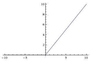
ReLU具有线性、非饱和性,而其非饱和性使得网络可以自行引入稀疏性。ReLU的使用解决了sigmoid梯度下降慢,深层网络的信息丢失的问题。ReLU在训练时是非常脆弱的,并且可能会“死”。例如,经过ReLU神经元的一个大梯度可能导致权重更新后该神经元接收到任何数据点都不会再激活。如果发生这种情况,之后通过该单位点的梯度将永远是零。也就是说,ReLU可能会在训练过程中不可逆地死亡,并且破坏数据流形。如果学习率太高,大部分网络将会“死亡”(即,在整个训练过程中神经元都没有激活)。而设置一个适当的学习率,可以在一定程度上避免这一问题。
6. 学习速率
上面说梯度下降的时候,说过学习速率其实就是梯度下降的步伐。因此,为了到达山谷,需要控制步伐的大小,即学习速率。学习速率大小的调节一般取决于 loss 的变化幅度。In [16]:# neural network with 5 layers
#
# · · · · · · · · · · (input data, flattened pixels) X [batch, 784] # 784 = 28*28
# \x/x\x/x\x/x\x/x\x/ -- fully connected layer (relu) W1 [784, 200] B1[200]
# · · · · · · · · · Y1 [batch, 200]
# \x/x\x/x\x/x\x/ -- fully connected layer (relu) W2 [200, 100] B2[100]
# · · · · · · · Y2 [batch, 100]
# \x/x\x/x\x/ -- fully connected layer (relu) W3 [100, 60] B3[60]
# · · · · · Y3 [batch, 60]
# \x/x\x/ -- fully connected layer (relu) W4 [60, 30] B4[30]
# · · · Y4 [batch, 30]
# \x/ -- fully connected layer (softmax) W5 [30, 10] B5[10]
# · Y5 [batch, 10]
model = Sequential()
model.add(Dense(200, input_shape=(784,)))#全连接,输入784维度, 输出10维度,需要和输入输出对应
model.add(Activation('relu'))# 将激活函数sigmoid改为ReLU
model.add(Dense(100))
model.add(Activation('relu'))
model.add(Dense(60))
model.add(Activation('relu'))
model.add(Dense(30))
model.add(Activation('relu'))
model.add(Dense(10))
model.add(Activation('softmax'))
sgd = Adam(lr=0.001)
model.compile(loss='binary_crossentropy',
optimizer=sgd,
metrics=['accuracy'])
#model 概要
model.summary()____________________________________________________________________________________________________ Layer (type) Output Shape Param # Connected to ==================================================================================================== dense_16 (Dense) (None, 200) 157000 dense_input_4[0][0] ____________________________________________________________________________________________________ activation_16 (Activation) (None, 200) 0 dense_16[0][0] ____________________________________________________________________________________________________ dense_17 (Dense) (None, 100) 20100 activation_16[0][0] ____________________________________________________________________________________________________ activation_17 (Activation) (None, 100) 0 dense_17[0][0] ____________________________________________________________________________________________________ dense_18 (Dense) (None, 60) 6060 activation_17[0][0] ____________________________________________________________________________________________________ activation_18 (Activation) (None, 60) 0 dense_18[0][0] ____________________________________________________________________________________________________ dense_19 (Dense) (None, 30) 1830 activation_18[0][0] ____________________________________________________________________________________________________ activation_19 (Activation) (None, 30) 0 dense_19[0][0] ____________________________________________________________________________________________________ dense_20 (Dense) (None, 10) 310 activation_19[0][0] ____________________________________________________________________________________________________ activation_20 (Activation) (None, 10) 0 dense_20[0][0] ==================================================================================================== Total params: 185,300 Trainable params: 185,300 Non-trainable params: 0 ____________________________________________________________________________________________________In [17]:
SVG(model_to_dot(model).create(prog='dot', format='svg'))Out[17]:dense_input_4: InputLayerdense_16: Denseactivation_16: Activationdense_17: Denseactivation_17: Activationdense_18: Denseactivation_18: Activationdense_19: Denseactivation_19: Activationdense_20: Denseactivation_20: ActivationIn [18]:
tensorboard3 = TensorBoard(log_dir='/home/tensorflow/log/five_layer_relu/epoch', histogram_freq=0)
my_tensorboard3 = BatchTensorBoard(log_dir='/home/tensorflow/log/five_layer_relu/batch')
model.fit(x_train_1, y_train_1,
nb_epoch=30,
verbose=0,
batch_size=100,
callbacks=[my_tensorboard3, tensorboard3])
Out[18]:
<keras.callbacks.History at 0xe3c6d50>In [19]:
#模型的测试误差指标
print(model.metrics_names)
# 对测试数据进行测试
model.evaluate(x_test_1, y_test_1,
verbose=1,
batch_size=100)
['loss', 'acc']
9600/10000 [===========================>..] - ETA: 0s
Out[19]:
[0.017244604945910281, 0.99598000288009647]
7.Dropout
运行目录下的mnist_2.1_five_layers_relu_lrdecay.py
随着迭代次数的增加,我们可以发现测试数据的loss值和训练数据的loss存在着巨大的差距, 随着迭代次数增加,train loss 越来越好,但test loss 的结果确越来越差,test loss 和 train loss 差距越来越大,模型开始过拟合。Dropout是指对于神经网络单元按照一定的概率将其暂时从网络中丢弃,从而解决过拟合问题。

可以对比mnist_2.1_five_layers_relu_lrdecay.py 和 加了dropout的/mnist_2.2_five_layers_relu_lrdecay_dropout.py的结果In [111]:
# neural network with 5 layers
#
# · · · · · · · · · ·       (input data, flattened pixels)       X [batch, 784]   # 784 = 28*28
# \x/x\x/x\x/x\x/x\x/ ✞  -- fully connected layer (relu+dropout) W1 [784, 200]      B1[200]
#  · · · · · · · · ·                                             Y1 [batch, 200]
#   \x/x\x/x\x/x\x/ ✞    -- fully connected layer (relu+dropout) W2 [200, 100]      B2[100]
#    · · · · · · ·                                               Y2 [batch, 100]
#    \x/x\x/x\x/ ✞       -- fully connected layer (relu+dropout) W3 [100, 60]       B3[60]
#     · · · · ·                                                  Y3 [batch, 60]
#     \x/x\x/ ✞          -- fully connected layer (relu+dropout) W4 [60, 30]        B4[30]
#      · · ·                                                     Y4 [batch, 30]
#      \x/               -- fully connected layer (softmax)      W5 [30, 10]        B5[10]
#       ·                                                        Y5 [batch, 10]
model = Sequential()
model.add(Dense(200, input_shape=(784,)))#全连接,输入784维度, 输出10维度,需要和输入输出对应
model.add(Activation('relu'))# 将激活函数sigmoid改为ReLU
model.add(Dense(100))
model.add(Activation('relu'))
model.add(Dropout(0.25))# 添加一个dropout层, 随机移除25%的单元
model.add(Dense(60))
model.add(Activation('relu'))
model.add(Dropout(0.25))
model.add(Dense(30))
model.add(Activation('relu'))
model.add(Dropout(0.25))
model.add(Dense(10))
model.add(Activation('softmax'))

sgd = Adam(lr=0.001)
model.compile(loss='binary_crossentropy',
optimizer=sgd,
metrics=['accuracy'])

#model 概要
model.summary()
____________________________________________________________________________________________________ Layer (type) Output Shape Param # Connected to ==================================================================================================== dense_171 (Dense) (None, 200) 157000 dense_input_35[0][0] ____________________________________________________________________________________________________ activation_171 (Activation) (None, 200) 0 dense_171[0][0] ____________________________________________________________________________________________________ dense_172 (Dense) (None, 100) 20100 activation_171[0][0] ____________________________________________________________________________________________________ activation_172 (Activation) (None, 100) 0 dense_172[0][0] ____________________________________________________________________________________________________ dropout_100 (Dropout) (None, 100) 0 activation_172[0][0] ____________________________________________________________________________________________________ dense_173 (Dense) (None, 60) 6060 dropout_100[0][0] ____________________________________________________________________________________________________ activation_173 (Activation) (None, 60) 0 dense_173[0][0] ____________________________________________________________________________________________________ dropout_101 (Dropout) (None, 60) 0 activation_173[0][0] ____________________________________________________________________________________________________ dense_174 (Dense) (None, 30) 1830 dropout_101[0][0] ____________________________________________________________________________________________________ activation_174 (Activation) (None, 30) 0 dense_174[0][0] ____________________________________________________________________________________________________ dropout_102 (Dropout) (None, 30) 0 activation_174[0][0] ____________________________________________________________________________________________________ dense_175 (Dense) (None, 10) 310 dropout_102[0][0] ____________________________________________________________________________________________________ activation_175 (Activation) (None, 10) 0 dense_175[0][0] ==================================================================================================== Total params: 185,300 Trainable params: 185,300 Non-trainable params: 0 ____________________________________________________________________________________________________In [112]:
SVG(model_to_dot(model).create(prog='dot', format='svg'))Out[112]:dense_input_35: InputLayerdense_171: Denseactivation_171: Activationdense_172: Denseactivation_172: Activationdropout_100: Dropoutdense_173: Denseactivation_173: Activationdropout_101: Dropoutdense_174: Denseactivation_174: Activationdropout_102: Dropoutdense_175: Denseactivation_175: ActivationIn [113]:
tensorboard4 = TensorBoard(log_dir='/home/tensorflow/log/five_layer_relu_dropout/epoch')
my_tensorboard4 = BatchTensorBoard(log_dir='/home/tensorflow/log/five_layer_relu_dropout/batch')

model.fit(x_train_1, y_train_1,
nb_epoch=30,
verbose=0,
batch_size=100,
callbacks=[tensorboard4, my_tensorboard4])
Out[113]:
<keras.callbacks.History at 0x27819610>In [114]:
#模型的测试误差指标
print(model.metrics_names)
# 对测试数据进行测试
model.evaluate(x_test_1, y_test_1,
verbose=1,
batch_size=100)
['loss', 'acc']
9900/10000 [============================>.] - ETA: 0s
Out[114]:
[0.025450729207368569, 0.99462999999523161]

相关文章推荐
- 基于Keras的深度学习的相关基础概念的讲解
- 基于Keras的深度学习的相关基础概念的讲解
- 基于Keras的深度学习的相关基础概念的讲解
- 基于Keras的深度学习的相关基础概念的讲解
- 基于Keras的深度学习的相关基础概念的讲解
- 基于Keras的深度学习的相关基础概念的讲解
- 基于Keras的深度学习的相关基础概念的讲解
- 基于Keras的深度学习的相关基础概念的讲解
- 基于Keras的深度学习的相关基础概念的讲解
- 基于Keras的深度学习的相关基础概念的讲解
- 基于Keras的深度学习的相关基础概念的讲解
- 基于Keras的深度学习的相关基础概念的讲解
- 基于Keras的深度学习的相关基础概念的讲解
- 基于Keras的深度学习的相关基础概念的讲解
- 基于Keras的深度学习的相关基础概念的讲解
- 基于keras的深度学习基本概念讲解
- 基于keras的深度学习基本概念讲解——深度学习之从小白到入门
- 基于keras的深度学习基本概念讲解——深度学习之从小白到入门
- 基于keras的深度学习基本概念讲解——深度学习之从小白到入门
- Logo 首页 下载App 深度学习从小白到入门 —— 基于keras的深度学习基本概念讲解 96 作者 shikanon 2017.02.18 20:27 字数 2551 阅读