Machine Learning|Andrew Ng|Coursera 吴恩达机器学习笔记
2018-02-08 11:28
393 查看
Week1:
Machine Learning:
A computer program is said to learn from experience E with respect to some class of tasks T and performance measure P, if its performance at tasks in T, as measured by P, improves with experience E.
Supervised Learning:We already know what our correct output should look like.
Regression:Try to map input variables to some continuous function.
Classification:Try to map input variables into discrete categories.
Unsupervised Learning:We only have little or no idea what our results should look like.
Clustering:Find a way to automatically group data into groups that are somehow similar or related by different variables.
Non-clustering:Find structure in a chaotic environment,like the "Cocktail Party Algorithm".
Model Representation:
x(i):Input features
y(i):Target variable
(x(i),y(i)):Training example
(x(i),y(i));i=1,...,m:Training set
m:Number of training examples
h(x):Hypothesis,θ0+θ1x1
Cost Function:This takes an average difference of all the results of the hypothesis with inputs from x's and the actual output y's.
Algorithm:

(The mean is halved 1/2 as a convenience for the computation of the gradient descent, as the derivative term of the square function will cancel out the 1/2 term.)
We use contour plot to show how to minimize the cost function.


Gradient Descent:Help us to estimate the parameters in the hypothesis function.
Algorithm:

(repeat until convergence)
j=0,1:Feature index numbe
α:Learning rate or the size of each step.If α is too small,gradient descent can be slow.If α is too large,gradient descent can overshoot the minimum.
Partial Derivative of J:Direction of each step
At each iteration j, one should simultaneously update all of the parameters.
Gradient Descent For Linear Regression:Algorithm:

This method looks at every example in the entire training set on every step, and is calledbatch gradient descent.
Linear Algebra:I have learned liner algebra in my college so I will skip this part in my note.
Week2:Mutiple Features:n:number of features
x(i):input of ith training example
x(i)j:value of feature j in ith training example
hθ(x):θ0x0+θ1x1+θ2x2+θ3x3+⋯+θnxn=

(assume x0 = 1)
Gradient Descent for Multiple Variables:
Algorithm:

Feature Scaling:
Feature Scaling:Dividing the input values by the range (max - min) of the input variable.Get every feature into approximately a -1 <= xi <= 1 range.
Mean Normalization:Subtracting the average value for an input variable from the values for that input variable resulting in a new average value for the input variable of just zero.

Where μi is the average of all the values for feature i and si is the range of values (max - min), or si is the standard deviation.
Learning Rate:Make a plot with number of iterations on the x-axis. and J(θ) on the y-axis.If J(θ) ever increases, then you probably need to decrease α.It has been proven that if learning rate α is sufficiently small, then J(θ) will decrease on every iteration.To choose α,try 0.001,0.003,0.01......
Features and Polynomial Regression:We can improve our features and the form of our hypothesis function in a couple different ways
We can combine multiple features into one.We can get a new feature x3 by taking x1 * x2
We can change the behavior or curve of our hypothesis function by making it a quadratic, cubic or square root function (or any other form).
if you choose your features this way then feature scaling becomes very important.
Normal Equation:Formula:

Example:

There is no need to do feature scaling with the normal equation.

If (X^TX) is non-invertibale:
Delete redundant features such as x1 = size in feet^2 and x2 = size in m^2.
Delete features to make sure that m > n or use regularization.
Octave:GNU Octave Docs
Vectorization can simplify the codes.
Week3:Classfication:The classification problem is just like the regression problem, except that the values we now want to predict take on only a small number of discrete values.
x(i):Feature
y(i):Label for the tranning example
Logistic Regression:We change the form for our hypotheses to satisfy 0 <= h(x) =1 by pluggin θ^Tx into the Logistic Function.
Formula:


Decision Boundary:The line that separates the area where y = 0 and where y = 1.It is created by hypothesis function(θ^Tx=0).
Cost Function:

We can compress our cost function's two conditional cases into one case:

Gradient De
10d53
scent:
This algorithm is identical to the one we used in linear regression.But the h(x) is changed.
Optimization Algorithms:
Conjugate gradient
BFGS
L-BGFS
We can write codes below to use Octave's "fminunc()"


Multiclass Classification:

Train a logistic regression classifier hθ(x) for each class to predict the probability that  y = i . To make a prediction on a new x, pick the class that maximizes hθ(x)
Overfitting:

Even though the fitted curve passes through the data perfectly, we would not expect this to be a very good predictor.
Options to address overfitting:
Reduce the number of features.
Regularzation.
Regularized Linear Regression:
Cost Funcion:

(lambda is the regularization parameter.)
Gradient Descent:


Normal Equation:

Regularized Logistic Regression:
Cost Function:

Gradient Descent:

Week4:Neural Network:Representation:

If we had one hidden layer, it would look like:

The values for each of the "activation" nodes:

Each layer gets its own matrix of weights:

(The '+1' comes from the 'bias nodes',the output nodes will not include the bias nodes while the inputs will.)
Vectorized:

We can set different theta matrix to construct fundamental options by using a small neural network.

We can construct more complex options by using hidden layers.

Multiclass Classification:We use one-vs-all method and let hypothesis function return a vector of values.
Week 5:Neural Network:Learning:Cost Function:
L:Total number of layers in the network
Sl:Number of units (not counting bias unit) in layer l
K:number of output units/classes

Backpropagation Algorithm:"Backpropagation" is neural-network terminology for minimizing our cost function.
Algorithm:For t = 1 to m:


We get

Using code like this to unroll all the elements and put them into one long vector.

Using code like this to get back original matrices.

Gradient Checking:We can approximate the derivative with respect to θj as follows:

Training:

Week 6:Applying Machine Learning:Evaluating a Hypothesis:Set 70% of date to be the training set and the remainning 30% to be the test set.

In order to choose the model of your hypothesis, we can test each degree of polynomial by using cross validation set.(20% training set,20% cross validation set,60% test set)

Bias vs. Variance:High bias is underfitting and high variance is overfitting.Ideally, we need to find a golden mean between these two.
High Bias:

High Variance:


In order to choose the model and the regularization term λ, we need to:

If a learning algorithm is suffering from high bias, getting more training data will not help much.
If a learning algorithm is suffering from high variance, getting more training data is likely to help.


A neural neural network with fewer parameters is prone to underfitting. It is also computationally cheaper.
A large neural network with more parameters is prone to overfitting. It is also computationally expensive.
Machine Learning System Desing:The recommended approach:
Start with a simple algorithm, implement it quickly, and test it early on your cross validation data.
Plot learning curves to decide if more data, more features, etc. are likely to help.
Manually examine the errors on examples in the cross validation set and try to spot a trend where most of the errors were made.
It is very important to get error results as a single, numerical value.
Precision
Handling Skewed Data:Skewed Classes:The ratio of positive to negative examples is very close to one of two extremes.

(y = 1 in presence of rare class that we want to detect)
Precision Rate:TP / (TP + FP)
Recall Rate:TP / (TP + FN)
F1 Score:(2 * P * R) / (P + R)
Week 7:Support Vector Machines:
Optimization Objective:

Because constant doesn't change value of the theta that achieves the miinmum,so we multiplying objective function in logistic regression by M.
We can both use (A + λB) or (CA + B) to control the relative.

A support vector machine just makes a prediction of y being equal to one or zero, directly. So the hypothesis will predict one
Large Margin Intuition:The SVM decision boundary will become like this:

The black line gives SVM a robustness because it has a large margin:

Kernels:Given (xi,yi),we choose li = xi as landmarks,then let fi = sim(x,li).
We compute new features depending on proximity to landmarks.So our function become theta0 + theta1*f1 + theta2*f2......
Gaussian Kernels:


C and Sigma:

Do perform feature scaling before using the Gaussian kernel.
Linear kernel:meanning no kernel.

Week8:Unsupervised Learning:
Clustering:
We give unlabeled training set to an algorithm and we ask the algorithm find some structure in the data for us.
K-meas Algorithm:
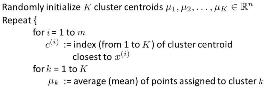
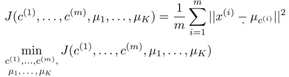
Cost Function:
Random Initialization:Randomly pick k training examples and set Mu1 of MuK equal to these k examples.
Elbow Method:
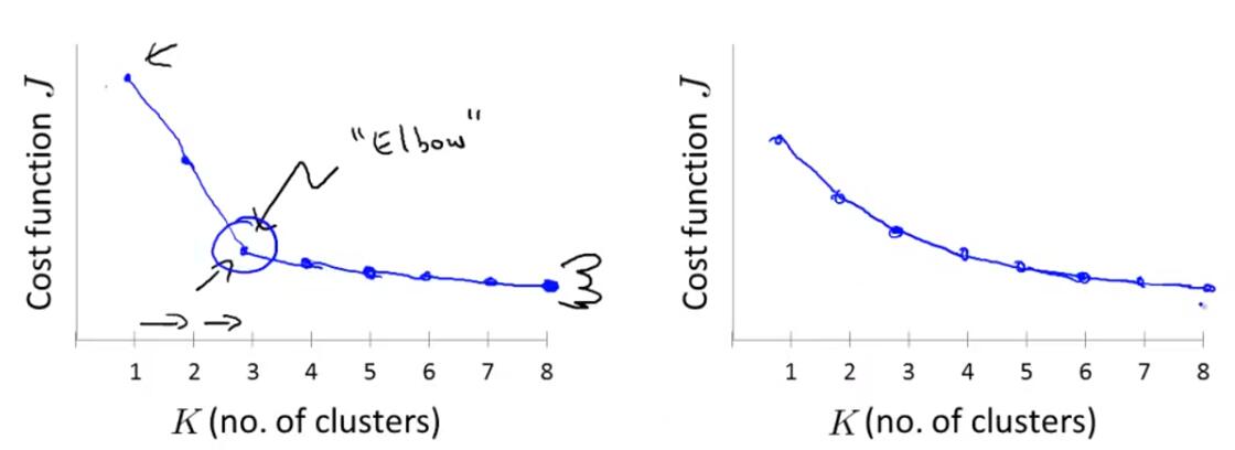
Better way to choose the number of clusters is to ask, for what purpose are you running K-means.
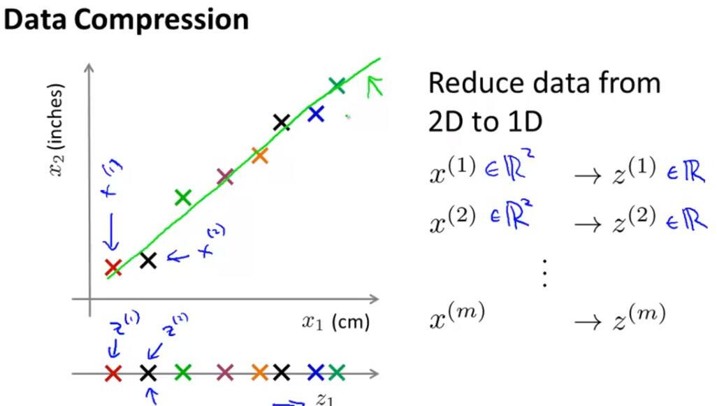
Dimensionality Reduction:Reason:Data compression or speed up our learning algorithm.
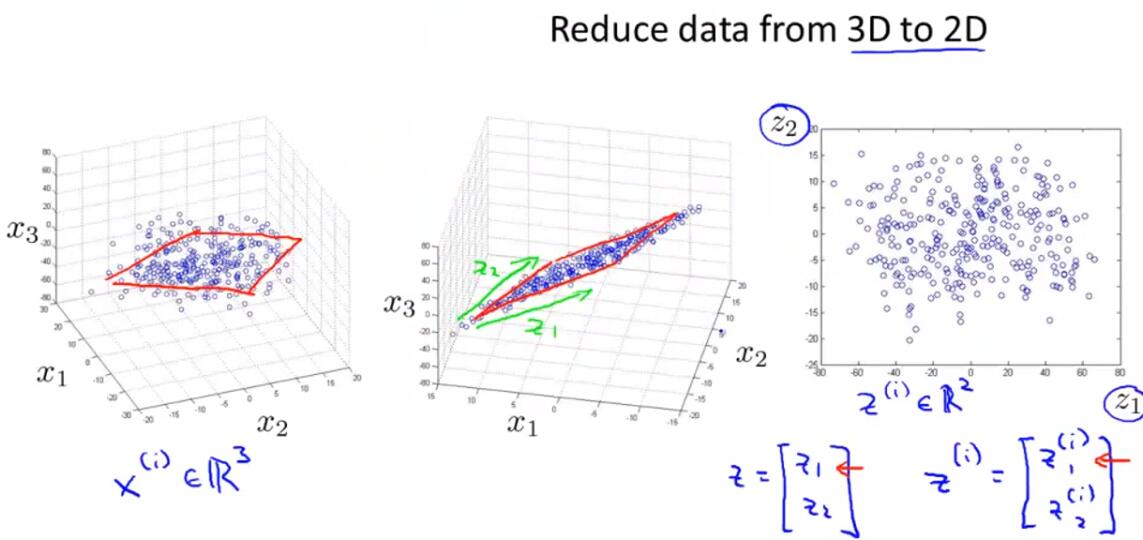
Visualization:We can use dimensionality reduction to reduce data from high dimensions down to 2 or 3 dimensions,so that we can plot it and understand our data better.
Principal Component Analysis:
PCA:Find a lower dimensional surface onto which to project the data, so as to minimize the square distance between each point and the location of where it gets projected.
Reduce from 2D to 1D:Find a vector onto which to project the data to minimize the projection error.
Reduce from nD to kD:Find k vectors onto which to project the data to minimize the projection error.
Data preprocessing:Feature scaling/Mean normalization
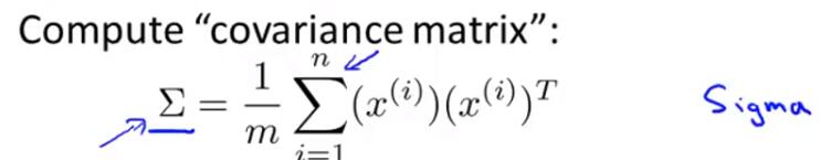
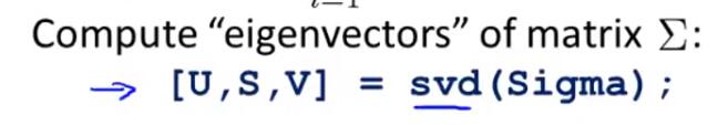
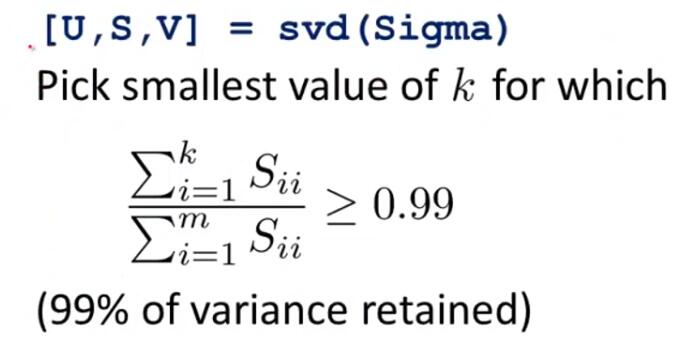
Algorithm:
If we want to reduce the data from n dimensions down to k dimensions, we need to do is take the first k vectors from U(n * n) as Ureduce(n * k).
z = Ureduce' * x.
Reconstruction from Compressed Representation:Xapprox = Ureduce * z.

Applying:
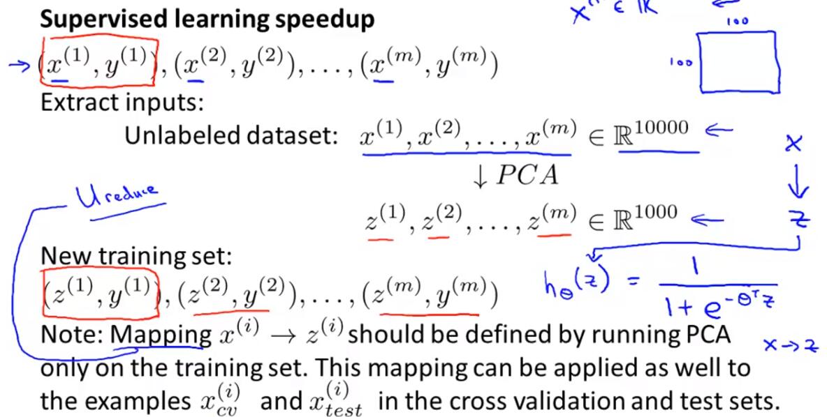
(Only if your algorithm doesn't do what you want then implement PCA)
Week 9:Anomaly Detection:
Density Estimation:
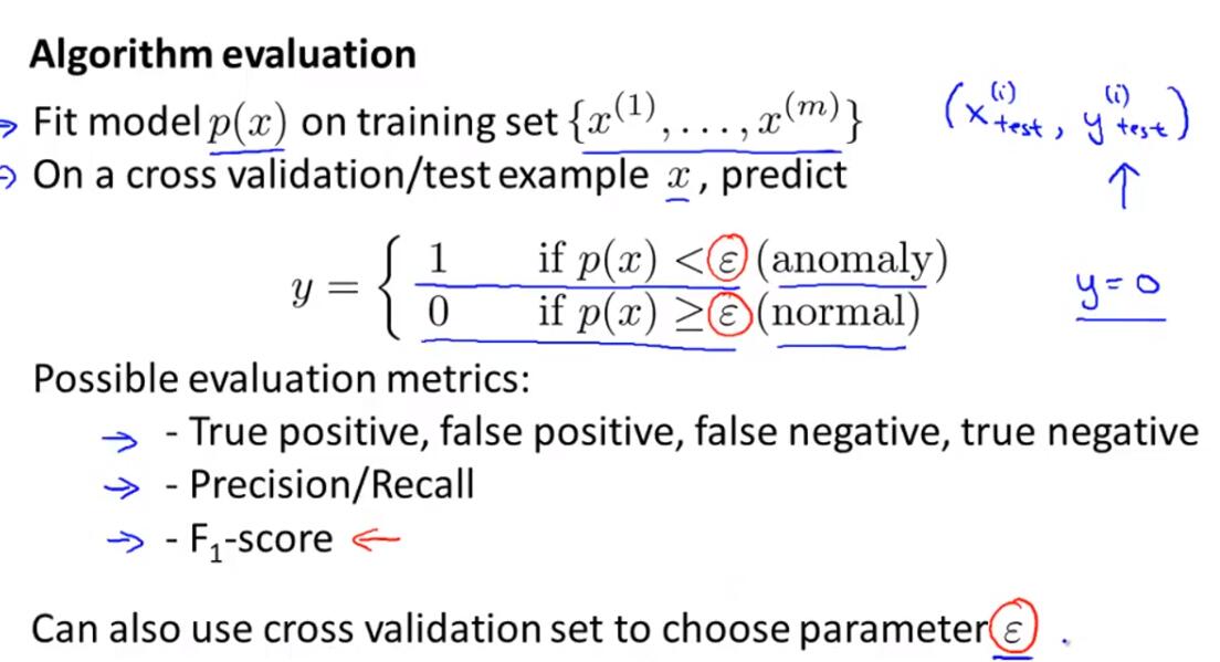
We build a model of the probability of x,if p of x-test is less than some epsilon then we flag this as an anomaly.
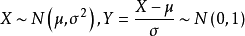
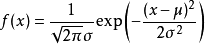
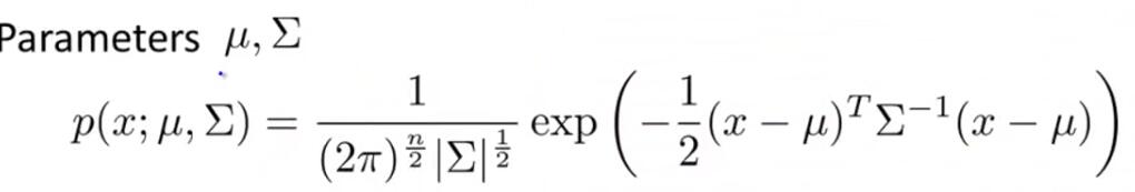
Gaussian Distribution(Normal Distribution):
,
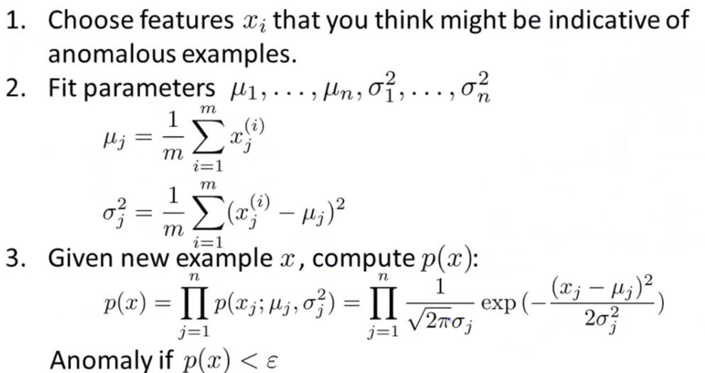
Parameter Estimation:

Algorithm:
Evaluation:Assume we have some labled data of anomalous and nonanomalous examples.Using training set(unlabled,assume normal examples),cross validation set and test set.
Anomaly Detection vs. Supervised Learning:

Non-gaussian Features:Let xNew = log(x)(logarithmic normal distribution),or xNew = x^(0.1)

Choose Features:Choose features that migth take on unusually large or small values in the event of an anomaly
Multivariate Gaussian Distribution:


Recommender Systems:
n.u = number of users
n.m = number of moives
r(i,j) = 1 if user j have rated movie i
y(i,j) = rating given by user j to movie i(only if r(i,j) = 1)
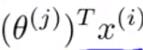
theta(j) = parameter vector for user j
x(i) = feature vector for movie i
Content Based Recommendations:
We assume we have features for different movies.
For each user j,learn a parameter.Predict user j as rating movie i with
stars.
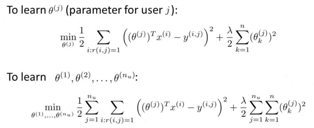
Optimization Objective:
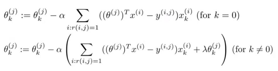
Gradient Descent:
Collaborative Filtering:
We assume that each of our users has told us how much they like the romantic movies and how much they like action packed movies.
Optimization Algorithm:
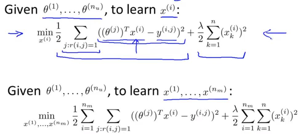
Given x and movie ratings can estimate theta.
Given theta and movie ratings can estimate x.
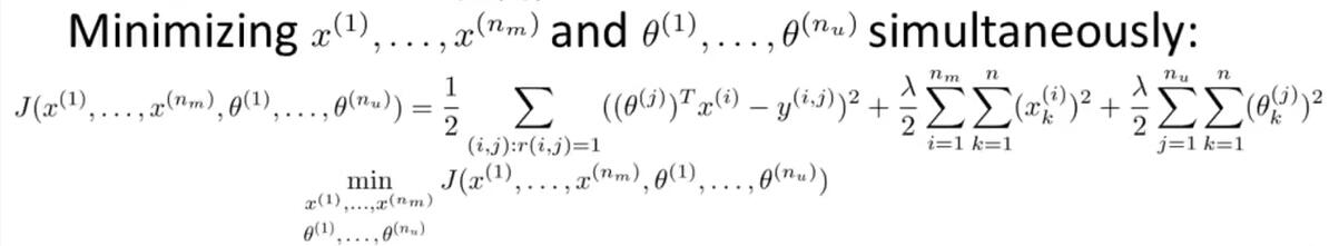
Optimization Objective:

Mean Normalization:Compute the average rating that each movie obtained and subtract off the meaning rating.So the rating of movie become
+ average rating.
Week 10:
Large Scale Machine Learning:
Stochastic Gradient Descent:
Algorithm:
Randomly shuffle the data set.
For i = 1...m:
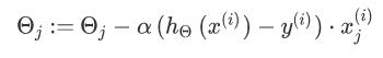
SGD will only try to fit one training example at a time. This way we can make progress in gradient descent without having to scan all m training examples first.
We will usually take 1-10 passes through data set to get near the global minimum.
Convergence:Plot the average cost of the hypothesis applied to every 1000 or so training examples. We can compute and save these costs during the gradient descent iterations.
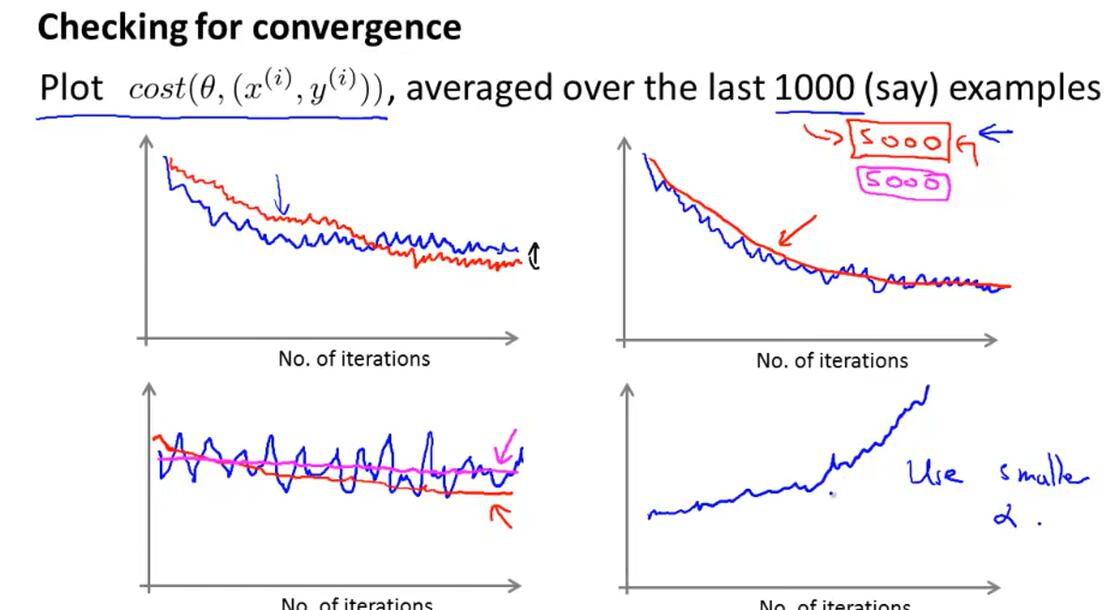
One strategy for trying to actually converge at the global minimum is to slowly decrease α over time.
Mini-Batch Gradient Descent:
Use b examples in each iteration.(b = mini-batch size)
Algorithm:

The advantage is that we can use vectorized implementations over the b examples.
Online Learning:
With a continuous stream of users to a website, we can run an endless loop that gets (x,y), where we collect some user actions for the features in x to predict some behavior y.
You can update θ for each individual (x,y) pair as you collect them. This way, you can adapt to new pools of users, since you are continuously updating theta.
Map Reduce and Data Parallelism:
Many learning algorithms can be expressed as computing sums of functions over the training set.
We can divide up batch gradient descent and dispatch the cost function for a subset of the data to many different machines so that we can train our algorithm in parallel.

Week 11:
Photo OCR:
Pipeline:
Text detection
Character segmentation
Character classification
Using sliding windows and expansion to text detection and character segmentation
Ceiling Analysis
Artificial Data Synthesis:
Creating new data from scratch(using the ramming funds as an example)
Taking existing label examples and introducing distortions to it, to sort of create extra label examples.

Machine Learning:
A computer program is said to learn from experience E with respect to some class of tasks T and performance measure P, if its performance at tasks in T, as measured by P, improves with experience E.
Supervised Learning:We already know what our correct output should look like.
Regression:Try to map input variables to some continuous function.
Classification:Try to map input variables into discrete categories.
Unsupervised Learning:We only have little or no idea what our results should look like.
Clustering:Find a way to automatically group data into groups that are somehow similar or related by different variables.
Non-clustering:Find structure in a chaotic environment,like the "Cocktail Party Algorithm".
Model Representation:
x(i):Input features
y(i):Target variable
(x(i),y(i)):Training example
(x(i),y(i));i=1,...,m:Training set
m:Number of training examples
h(x):Hypothesis,θ0+θ1x1
Cost Function:This takes an average difference of all the results of the hypothesis with inputs from x's and the actual output y's.
Algorithm:
(The mean is halved 1/2 as a convenience for the computation of the gradient descent, as the derivative term of the square function will cancel out the 1/2 term.)
We use contour plot to show how to minimize the cost function.
Gradient Descent:Help us to estimate the parameters in the hypothesis function.
Algorithm:
(repeat until convergence)
j=0,1:Feature index numbe
α:Learning rate or the size of each step.If α is too small,gradient descent can be slow.If α is too large,gradient descent can overshoot the minimum.
Partial Derivative of J:Direction of each step
At each iteration j, one should simultaneously update all of the parameters.
Gradient Descent For Linear Regression:Algorithm:
This method looks at every example in the entire training set on every step, and is calledbatch gradient descent.
Linear Algebra:I have learned liner algebra in my college so I will skip this part in my note.
Week2:Mutiple Features:n:number of features
x(i):input of ith training example
x(i)j:value of feature j in ith training example
hθ(x):θ0x0+θ1x1+θ2x2+θ3x3+⋯+θnxn=
(assume x0 = 1)
Gradient Descent for Multiple Variables:
Algorithm:
Feature Scaling:
Feature Scaling:Dividing the input values by the range (max - min) of the input variable.Get every feature into approximately a -1 <= xi <= 1 range.
Mean Normalization:Subtracting the average value for an input variable from the values for that input variable resulting in a new average value for the input variable of just zero.
Where μi is the average of all the values for feature i and si is the range of values (max - min), or si is the standard deviation.
Learning Rate:Make a plot with number of iterations on the x-axis. and J(θ) on the y-axis.If J(θ) ever increases, then you probably need to decrease α.It has been proven that if learning rate α is sufficiently small, then J(θ) will decrease on every iteration.To choose α,try 0.001,0.003,0.01......
Features and Polynomial Regression:We can improve our features and the form of our hypothesis function in a couple different ways
We can combine multiple features into one.We can get a new feature x3 by taking x1 * x2
We can change the behavior or curve of our hypothesis function by making it a quadratic, cubic or square root function (or any other form).
if you choose your features this way then feature scaling becomes very important.
Normal Equation:Formula:
Example:
There is no need to do feature scaling with the normal equation.
If (X^TX) is non-invertibale:
Delete redundant features such as x1 = size in feet^2 and x2 = size in m^2.
Delete features to make sure that m > n or use regularization.
Octave:GNU Octave Docs
Vectorization can simplify the codes.
Week3:Classfication:The classification problem is just like the regression problem, except that the values we now want to predict take on only a small number of discrete values.
x(i):Feature
y(i):Label for the tranning example
Logistic Regression:We change the form for our hypotheses to satisfy 0 <= h(x) =1 by pluggin θ^Tx into the Logistic Function.
Formula:
Decision Boundary:The line that separates the area where y = 0 and where y = 1.It is created by hypothesis function(θ^Tx=0).
Cost Function:
We can compress our cost function's two conditional cases into one case:
Gradient De
10d53
scent:
This algorithm is identical to the one we used in linear regression.But the h(x) is changed.
Optimization Algorithms:
Conjugate gradient
BFGS
L-BGFS
We can write codes below to use Octave's "fminunc()"
Multiclass Classification:
Train a logistic regression classifier hθ(x) for each class to predict the probability that  y = i . To make a prediction on a new x, pick the class that maximizes hθ(x)
Overfitting:
Even though the fitted curve passes through the data perfectly, we would not expect this to be a very good predictor.
Options to address overfitting:
Reduce the number of features.
Regularzation.
Regularized Linear Regression:
Cost Funcion:
(lambda is the regularization parameter.)
Gradient Descent:
Normal Equation:
Regularized Logistic Regression:
Cost Function:
Gradient Descent:
Week4:Neural Network:Representation:
If we had one hidden layer, it would look like:
The values for each of the "activation" nodes:
Each layer gets its own matrix of weights:
(The '+1' comes from the 'bias nodes',the output nodes will not include the bias nodes while the inputs will.)
Vectorized:
We can set different theta matrix to construct fundamental options by using a small neural network.
We can construct more complex options by using hidden layers.
Multiclass Classification:We use one-vs-all method and let hypothesis function return a vector of values.
Week 5:Neural Network:Learning:Cost Function:
L:Total number of layers in the network
Sl:Number of units (not counting bias unit) in layer l
K:number of output units/classes
Backpropagation Algorithm:"Backpropagation" is neural-network terminology for minimizing our cost function.
Algorithm:For t = 1 to m:
We get
Using code like this to unroll all the elements and put them into one long vector.
Using code like this to get back original matrices.
Gradient Checking:We can approximate the derivative with respect to θj as follows:
Training:
Week 6:Applying Machine Learning:Evaluating a Hypothesis:Set 70% of date to be the training set and the remainning 30% to be the test set.
In order to choose the model of your hypothesis, we can test each degree of polynomial by using cross validation set.(20% training set,20% cross validation set,60% test set)
Bias vs. Variance:High bias is underfitting and high variance is overfitting.Ideally, we need to find a golden mean between these two.
High Bias:
High Variance:
In order to choose the model and the regularization term λ, we need to:
If a learning algorithm is suffering from high bias, getting more training data will not help much.
If a learning algorithm is suffering from high variance, getting more training data is likely to help.
A neural neural network with fewer parameters is prone to underfitting. It is also computationally cheaper.
A large neural network with more parameters is prone to overfitting. It is also computationally expensive.
Machine Learning System Desing:The recommended approach:
Start with a simple algorithm, implement it quickly, and test it early on your cross validation data.
Plot learning curves to decide if more data, more features, etc. are likely to help.
Manually examine the errors on examples in the cross validation set and try to spot a trend where most of the errors were made.
It is very important to get error results as a single, numerical value.
Precision
Handling Skewed Data:Skewed Classes:The ratio of positive to negative examples is very close to one of two extremes.
(y = 1 in presence of rare class that we want to detect)
Precision Rate:TP / (TP + FP)
Recall Rate:TP / (TP + FN)
F1 Score:(2 * P * R) / (P + R)
Week 7:Support Vector Machines:
Optimization Objective:
Because constant doesn't change value of the theta that achieves the miinmum,so we multiplying objective function in logistic regression by M.
We can both use (A + λB) or (CA + B) to control the relative.
A support vector machine just makes a prediction of y being equal to one or zero, directly. So the hypothesis will predict one
Large Margin Intuition:The SVM decision boundary will become like this:
The black line gives SVM a robustness because it has a large margin:
Kernels:Given (xi,yi),we choose li = xi as landmarks,then let fi = sim(x,li).
We compute new features depending on proximity to landmarks.So our function become theta0 + theta1*f1 + theta2*f2......
Gaussian Kernels:
C and Sigma:
Do perform feature scaling before using the Gaussian kernel.
Linear kernel:meanning no kernel.
Week8:Unsupervised Learning:
Clustering:
We give unlabeled training set to an algorithm and we ask the algorithm find some structure in the data for us.
K-meas Algorithm:
Cost Function:
Random Initialization:Randomly pick k training examples and set Mu1 of MuK equal to these k examples.
Elbow Method:
Better way to choose the number of clusters is to ask, for what purpose are you running K-means.
Dimensionality Reduction:Reason:Data compression or speed up our learning algorithm.
Visualization:We can use dimensionality reduction to reduce data from high dimensions down to 2 or 3 dimensions,so that we can plot it and understand our data better.
Principal Component Analysis:
PCA:Find a lower dimensional surface onto which to project the data, so as to minimize the square distance between each point and the location of where it gets projected.
Reduce from 2D to 1D:Find a vector onto which to project the data to minimize the projection error.
Reduce from nD to kD:Find k vectors onto which to project the data to minimize the projection error.
Data preprocessing:Feature scaling/Mean normalization
Algorithm:
If we want to reduce the data from n dimensions down to k dimensions, we need to do is take the first k vectors from U(n * n) as Ureduce(n * k).
z = Ureduce' * x.
Reconstruction from Compressed Representation:Xapprox = Ureduce * z.
Applying:
(Only if your algorithm doesn't do what you want then implement PCA)
Week 9:Anomaly Detection:
Density Estimation:
We build a model of the probability of x,if p of x-test is less than some epsilon then we flag this as an anomaly.
Gaussian Distribution(Normal Distribution):
,
Parameter Estimation:
Algorithm:
Evaluation:Assume we have some labled data of anomalous and nonanomalous examples.Using training set(unlabled,assume normal examples),cross validation set and test set.
Anomaly Detection vs. Supervised Learning:
Non-gaussian Features:Let xNew = log(x)(logarithmic normal distribution),or xNew = x^(0.1)
Choose Features:Choose features that migth take on unusually large or small values in the event of an anomaly
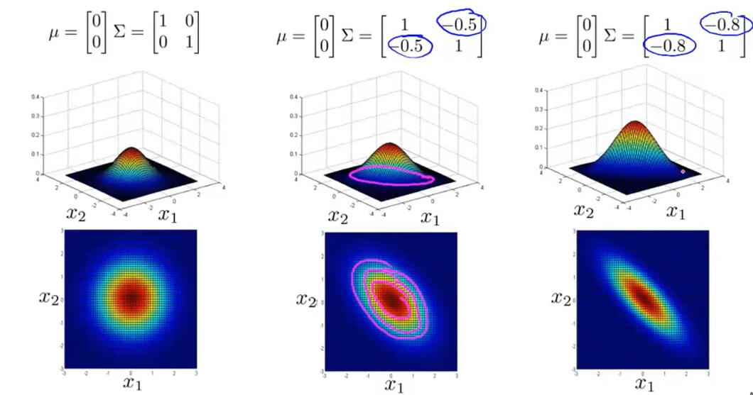
Multivariate Gaussian Distribution:
Recommender Systems:
n.u = number of users
n.m = number of moives
r(i,j) = 1 if user j have rated movie i
y(i,j) = rating given by user j to movie i(only if r(i,j) = 1)
theta(j) = parameter vector for user j
x(i) = feature vector for movie i
Content Based Recommendations:
We assume we have features for different movies.
For each user j,learn a parameter.Predict user j as rating movie i with
stars.
Optimization Objective:
Gradient Descent:
Collaborative Filtering:
We assume that each of our users has told us how much they like the romantic movies and how much they like action packed movies.
Optimization Algorithm:
Given x and movie ratings can estimate theta.
Given theta and movie ratings can estimate x.
Optimization Objective:
Mean Normalization:Compute the average rating that each movie obtained and subtract off the meaning rating.So the rating of movie become
+ average rating.
Week 10:
Large Scale Machine Learning:
Stochastic Gradient Descent:
Algorithm:
Randomly shuffle the data set.
For i = 1...m:
SGD will only try to fit one training example at a time. This way we can make progress in gradient descent without having to scan all m training examples first.
We will usually take 1-10 passes through data set to get near the global minimum.
Convergence:Plot the average cost of the hypothesis applied to every 1000 or so training examples. We can compute and save these costs during the gradient descent iterations.
One strategy for trying to actually converge at the global minimum is to slowly decrease α over time.
Mini-Batch Gradient Descent:
Use b examples in each iteration.(b = mini-batch size)
Algorithm:
The advantage is that we can use vectorized implementations over the b examples.
Online Learning:
With a continuous stream of users to a website, we can run an endless loop that gets (x,y), where we collect some user actions for the features in x to predict some behavior y.
You can update θ for each individual (x,y) pair as you collect them. This way, you can adapt to new pools of users, since you are continuously updating theta.
Map Reduce and Data Parallelism:
Many learning algorithms can be expressed as computing sums of functions over the training set.
We can divide up batch gradient descent and dispatch the cost function for a subset of the data to many different machines so that we can train our algorithm in parallel.
Week 11:
Photo OCR:
Pipeline:
Text detection
Character segmentation
Character classification
Using sliding windows and expansion to text detection and character segmentation
Ceiling Analysis
Artificial Data Synthesis:
Creating new data from scratch(using the ramming funds as an example)
Taking existing label examples and introducing distortions to it, to sort of create extra label examples.

相关文章推荐
- coursera上的Andrew Ng机器学习笔记1
- 吴恩达Coursera深度学习课程 DeepLearning.ai 提炼笔记(3-1)-- 机器学习策略(1)(转)
- Coursera-吴恩达-机器学习-(第4周笔记)Neural Networks——Representation
- coursera-斯坦福-机器学习-吴恩达-第11周笔记-ORC系统
- 吴恩达Coursera深度学习课程 DeepLearning.ai 提炼笔记(3-2)-- 机器学习策略(2)(转)
- Coursera机器学习(Andrew Ng)笔记:大规模机器学习
- Coursera-吴恩达-机器学习-(第11周笔记)应用实例:photo OCR
- Coursera-吴恩达-机器学习-(第2周笔记)Linear Regression with Multiple Variables
- COURSERA 机器学习课笔记(by Prof. Andrew Ng)学习笔记(一)
- Coursera 机器学习(by Andrew Ng)课程学习笔记 Week 4——神经网络(一)
- coursera-斯坦福-机器学习-吴恩达-第3周笔记-逻辑回归
- Coursera-吴恩达-机器学习-(第3周笔记)Logistic Regression and Regularization
- Coursera 机器学习(by Andrew Ng)课程学习笔记 Week 9(二)——推荐系统作业
- Coursera 机器学习(by Andrew Ng)课程学习笔记 Week 5——神经网络(二)
- Coursera机器学习(Andrew Ng)笔记:回归与分类问题
- 吴恩达Coursera机器学习课程笔记-单变量线性回归
- Coursera 机器学习(by Andrew Ng)课程学习笔记 Week 6(一)—— 机器学习诊断、偏差与方差
- Coursera 机器学习(by Andrew Ng)课程学习笔记 Week 3——逻辑回归、过拟合与正则化
- 课程笔记|吴恩达Coursera机器学习 Week1 笔记-机器学习基础
- 机器学习(Machine Learning)- 吴恩达(Andrew Ng )-笔记