使用 Caffe Python 编写 LeNet

使用 Caffe Python 编写 LeNet

前言:

本文翻译自 Solving in Python with LeNet，基于深度学习框架 Caffe 的应用，运行本代码的前提是：

安装了Caffe，windows Caffe安装教程以及添加Python接口请参考Caffe安装 和编译Caffe Python接口

安装 Python 2.7，推荐使用Anaconda安装。安装完以后启动Jupyter Notebook

注：为正确运行程序，本文代码对原文代码有改动。

还有，代码中的细节我会在详解目录中陆续更新

详解目录

caffe.NetSpec()

Caffe solver.net.forward()，solver.test_nets[0].forward() 和 solver.step(1)

正文：

1. 开始 （Setup）

导入 pylab，画图使用。

from pylab import *

导入 caffe，添加系统变量。

caffe_root = 'D:/wincaffe/caffe-master/'  # 这是我的caffe 根目录

import sys
sys.path.insert(0, caffe_root + 'python')
import caffe

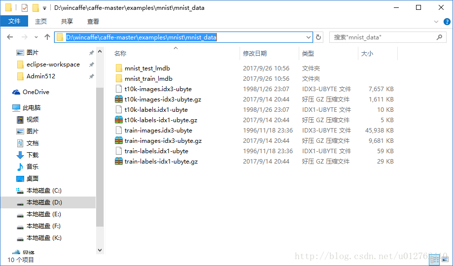
下载数据，下载好的数据请放在 D:\wincaffe\caffe-master\examples\mnist\mnist_data 目录下，我使用的是绝对路径。mnist 二进制文件需要转换为lmdb格式，我将原mnist文件和 lmdb 文件放在百度网盘mnist+lmdb (密码：h7wh)上了，不会转换的可以下载。

2.创建网络（Creating the net）

现在我们创建一个源自1989年的经典卷积网络结构 LeNet 的变体。

我们需要两个额外的文件方便输出：

net prototxt：定义了指向 train/test 数据的网络结构。

solver prototxt : 定义了网络学习参数。

from caffe import layers as L, params as P
def lenet(lmdb, batch_size):
# our version of LeNet: a series of linear and simple nonlinear transformations
n = caffe.NetSpec() # 见详解目录-1

n.data, n.label = L.Data(batch_size=batch_size, backend=P.Data.LMDB, source=lmdb,
transform_param=dict(scale=1./255), ntop=2)

n.conv1 = L.Convolution(n.data, kernel_size=5, num_output=20, weight_filler=dict(type='xavier'))
n.pool1 = L.Pooling(n.conv1, kernel_size=2, stride=2, pool=P.Pooling.MAX)
n.conv2 = L.Convolution(n.pool1, kernel_size=5, num_output=50, weight_filler=dict(type='xavier'))
n.pool2 = L.Pooling(n.conv2, kernel_size=2, stride=2, pool=P.Pooling.MAX)
n.fc1 =   L.InnerProduct(n.pool2, num_output=500, weight_filler=dict(type='xavier'))
n.relu1 = L.ReLU(n.fc1, in_place=True)
n.score = L.InnerProduct(n.relu1, num_output=10, weight_filler=dict(type='xavier'))
n.loss =  L.SoftmaxWithLoss(n.score, n.label)

return n.to_proto() #写入到prototxt文件

with open('D:/wincaffe/caffe-master/examples/mnist/lenet_auto_train.prototxt', 'w') as f:
f.write(str(lenet('D:/wincaffe/caffe-master/examples/mnist/mnist_data/mnist_train_lmdb', 64)))

with open('D:/wincaffe/caffe-master/examples/mnist/lenet_auto_test.prototxt', 'w') as f:
f.write(str(lenet('D:/wincaffe/caffe-master/examples/mnist/mnist_data/mnist_test_lmdb', 100)))

让我们看一下 train net 的结构:

layer {
name: "data"
type: "Data"
top: "data"
top: "label"
transform_param {
scale: 0.00392156862745
}
data_param {
source: "D:/wincaffe/caffe-master/examples/mnist/mnist_data/mnist_train_lmdb"
batch_size: 64
backend: LMDB
}
}
layer {
name: "conv1"
type: "Convolution"
bottom: "data"
top: "conv1"
convolution_param {
num_output: 20
kernel_size: 5
weight_filler {
type: "xavier"
}
}
}
layer {
name: "pool1"
type: "Pooling"
bottom: "conv1"
top: "pool1"
pooling_param {
pool: MAX
kernel_size: 2
stride: 2
}
}
layer {
name: "conv2"
type: "Convolution"
bottom: "pool1"
top: "conv2"
convolution_param {
num_output: 50
kernel_size: 5
weight_filler {
type: "xavier"
}
}
}
layer {
name: "pool2"
type: "Pooling"
bottom: "conv2"
top: "pool2"
pooling_param {
pool: MAX
kernel_size: 2
stride: 2
}
}
layer {
name: "fc1"
type: "InnerProduct"
bottom: "pool2"
top: "fc1"
inner_product_param {
num_output: 500
weight_filler {
type: "xavier"
}
}
}
layer {
name: "relu1"
type: "ReLU"
bottom: "fc1"
top: "fc1"
}
layer {
name: "score"
type: "InnerProduct"
bottom: "fc1"
top: "score"
inner_product_param {
num_output: 10
weight_filler {
type: "xavier"
}
}
}
layer {
name: "loss"
type: "SoftmaxWithLoss"
bottom: "score"
bottom: "label"
top: "loss"
}

还有 test net 的结构:

layer {
name: "data"
type: "Data"
top: "data"
top: "label"
transform_param {
scale: 0.00392156862745
}
data_param {
source: "D:/wincaffe/caffe-master/examples/mnist/mnist_data/mnist_test_lmdb"
batch_size: 100
backend: LMDB
}
}
layer {
name: "conv1"
type: "Convolution"
bottom: "data"
top: "conv1"
convolution_param {
num_output: 20
kernel_size: 5
weight_filler {
type: "xavier"
}
}
}
layer {
name: "pool1"
type: "Pooling"
bottom: "conv1"
top: "pool1"
pooling_param {
pool: MAX
kernel_size: 2
stride: 2
}
}
layer {
name: "conv2"
type: "Convolution"
bottom: "pool1"
top: "conv2"
convolution_param {
num_output: 50
kernel_size: 5
weight_filler {
type: "xavier"
}
}
}
layer {
name: "pool2"
type: "Pooling"
bottom: "conv2"
top: "pool2"
pooling_param {
pool: MAX
kernel_size: 2
stride: 2
}
}
layer {
name: "fc1"
type: "InnerProduct"
bottom: "pool2"
top: "fc1"
inner_product_param {
num_output: 500
weight_filler {
type: "xavier"
}
}
}
layer {
name: "relu1"
type: "ReLU"
bottom: "fc1"
top: "fc1"
}
layer {
name: "score"
type: "InnerProduct"
bottom: "fc1"
top: "score"
inner_product_param {
num_output: 10
weight_filler {
type: "xavier"
}
}
}
layer {
name: "loss"
type: "SoftmaxWithLoss"
bottom: "score"
bottom: "label"
top: "loss"
}

嗯，再给你看看solver的结构。这个文件在 D:\wincaffe\caffe-master\examples\mnist 中本来就存在。不过你需要根据路径自己修改一下代码中 train_net，test_net的路径。

# The train/test net protocol buffer definition
train_net: "D:/wincaffe/caffe-master/examples/mnist/lenet_auto_train.prototxt"
test_net: "D:/wincaffe/caffe-master/examples/mnist/lenet_auto_test.prototxt"
# test_iter specifies how many forward passes the test should carry out.
# In the case of MNIST, we have test batch size 100 and 100 test iterations,
# covering the full 10,000 testing images.
test_iter: 100
# Carry out testing every 500 training iterations.
test_interval: 500
# The base learning rate, momentum and the weight decay of the network.
base_lr: 0.01
momentum: 0.9
weight_decay: 0.0005
# The learning rate policy
lr_policy: "inv"
gamma: 0.0001
power: 0.75
# Display every 100 iterations
display: 100
# The maximum number of iterations
max_iter: 10000
# snapshot intermediate results
snapshot: 5000
snapshot_prefix: "mnist/lenet"

3.加载和验证solver（Loading and checking the solver）

译者注：选择设备和使用GPU。（没有安装CUDA+cuDnn的可以使用caffe.set_mode_cpu()，亲测，速度慢成屎。）

caffe.set_device(0) #选择默认gpu
caffe.set_mode_gpu()    #使用gpu

### load the solver and create train and test nets
solver = None  # ignore this workaround for lmdb data (can't instantiate two solvers on the same data)
solver = caffe.SGDSolver('C:/Users/Admin512/Desktop/MyStudy/caffe_python/LeNet/mnist/lenet_auto_solver.prototxt')

看一下中间变量的维度：

代码1：

# each output is (batch size, feature dim, spatial dim)
[(k, v.data.shape) for k, v in solver.net.blobs.items()]

输出1：

[('data', (64L, 1L, 28L, 28L)),
('label', (64L,)),
('conv1', (64L, 20L, 24L, 24L)),
('pool1', (64L, 20L, 12L, 12L)),
('conv2', (64L, 50L, 8L, 8L)),
('pool2', (64L, 50L, 4L, 4L)),
('fc1', (64L, 500L)),
('score', (64L, 10L)),
('loss', ())]

代码2：

# just print the weight sizes (we'll omit the biases)
[(k, v[0].data.shape) for k, v in solver.net.params.items()]

输出2：

[('conv1', (20, 1, 5, 5)),
('conv2', (50, 20, 5, 5)),
('fc1', (500, 800)),
('score', (10, 500))]

训练前，让我们检查一下是否一切就绪：

代码1：

# 见详解目录-2
solver.net.forward()  # train net
solver.test_nets[0].forward()  # test net (there can be more than one)

输出1：

{'loss': array(2.365971088409424, dtype=float32)}

代码2：

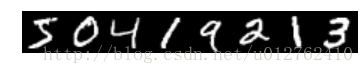
# we use a little trick to tile the first eight images
imshow(solver.net.blobs['data'].data[:8, 0].transpose(1, 0, 2).reshape(28, 8*28), cmap='gray'); axis('off')
print 'train labels:', solver.net.blobs['label'].data[:8]

输出2：

train labels: [ 5.  0.  4.  1.  9.  2.  1.  3.]

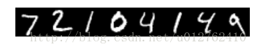
代码3：

imshow(solver.test_nets[0].blobs['data'].data[:8, 0].transpose(1, 0, 2).reshape(28, 8*28), cmap='gray'); axis('off')
print 'test labels:', solver.test_nets[0].blobs['label'].data[:8]

输出3：

test labels: [ 7.  2.  1.  0.  4.  1.  4.  9.]

4.做一步solver（Stepping the solver）

训练网络和测试网看起来都在加载数据，并拥有正确的标签。

让我们做一步 minibatch-SGD ，看一下发生了什么：

# 见详解目录-2
solver.step(1)

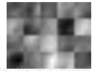
我们通过我们的滤波器（filters）进行了梯度传播吗？让我们看一下第一层的更新，这里展示了5×5的滤波器组成的4×5的网格。

代码4：

imshow(solver.net.params['conv1'][0].diff[:, 0].reshape(4, 5, 5, 5)
.transpose(0, 2, 1, 3).reshape(4*5, 5*5), cmap='gray'); axis('off')

输出4：

(-0.5, 24.5, 19.5, -0.5)

5.编写一个自定义的训练循环（Writing a custom training loop）

Something is happening. 我们让网络运行一段时间，运行期间我们保持跟踪一些事情。注意，这个过程和通过caffe二进制训练一样。特别是：

日志记录将继续正常进行。

在solver prototxt 指定的间隔获取快照（在这里，间隔取5000次迭代）

在指定的间隔进行测试（在这里，间隔取500次迭代）

因为我们可以使用 Python 控制循环，我们可以自由的计算额外的东西，就像下面展示的一样。我们也可以做一些别的事情，比如：

写一个自定义的停止标准

通过更新循环中的网络来改变求解过程

代码5：

%%time
niter = 200
test_interval = 25
# losses will also be stored in the log
train_loss = zeros(niter)
test_acc = zeros(int(np.ceil(niter / test_interval)))
output = zeros((niter, 8, 10))

# the main solver loop
for it in range(niter):
solver.step(1)  # SGD by Caffe

# store the train loss
train_loss[it] = solver.net.blobs['loss'].data

# store the output on the first test batch
# (start the forward pass at conv1 to avoid loading new data)
solver.test_nets[0].forward(start='conv1')
output[it] = solver.test_nets[0].blobs['score'].data[:8]

# run a full test every so often
# (Caffe can also do this for us and write to a log, but we show here
#  how to do it directly in Python, where more complicated things are easier.)
if it % test_interval == 0:
print 'Iteration', it, 'testing...'
correct = 0
for test_it in range(100):
solver.test_nets[0].forward()
correct += sum(solver.test_nets[0].blobs['score'].data.argmax(1)
== solver.test_nets[0].blobs['label'].data)
test_acc[it // test_interval] = correct / 1e4

输出5：

（貌似我的GPU比他们的好不少！）

Iteration 0 testing...
Iteration 25 testing...
Iteration 50 testing...
Iteration 75 testing...
Iteration 100 testing...
Iteration 125 testing...
Iteration 150 testing...
Iteration 175 testing...
Wall time: 2.3 s

我们看一下训练损失函数和测试正确率

代码6：

_, ax1 = subplots()
ax2 = ax1.twinx()
ax1.plot(arange(niter), train_loss)
ax2.plot(test_interval * arange(len(test_acc)), test_acc, 'r')
ax1.set_xlabel('iteration')
ax1.set_ylabel('train loss')
ax2.set_ylabel('test accuracy')
ax2.set_title('Test Accuracy: {:.2f}'.format(test_acc[-1]))

输出6：

<matplotlib.text.Text at 0x32b3fb38>

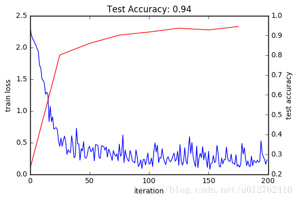
损失函数下降的很快，而且收敛（except for stochasticity，我觉得这句话翻译成除了局部随机性），相应的，正确率在上升。Hooray!

因为我们在第一次测试batch中保存了结果，所以我们可以观察我们的预测分数是如何演变的。x轴是迭代次数，y轴是标签。

代码7：

for i in range(8):
figure(figsize=(2, 2))
imshow(solver.test_nets[0].blobs['data'].data[i, 0], cmap='gray')
figure(figsize=(10, 2))
imshow(output[:50, i].T, interpolation='nearest', cmap='gray')
xlabel('iteration')
ylabel('label')

输出7：



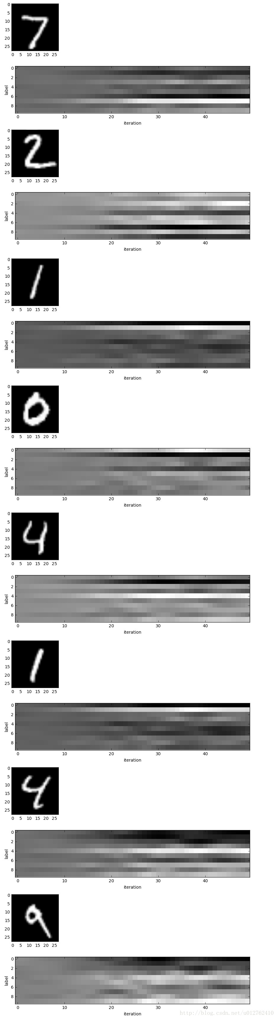
我们刚开始对这些数字（digit）一点都不了解，但是最后我们对每个数字都有正确的分类。随着分类的进行，你会发现识别最后的数字是非常困难的，倾斜的“9”很容易和“4”混淆。

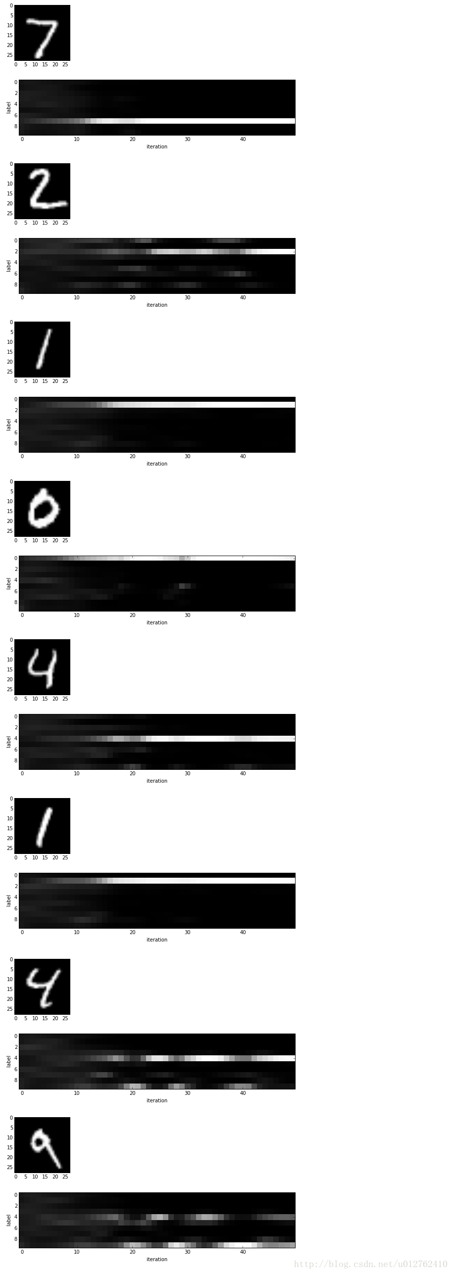
注意：以上都是原始的输出而不是 softmax 计算的概率向量。如下所示，后者很容易表示我们的网络的 confidence （但是很难看到难以识别数字的分数）。

代码8：

for i in range(8):
figure(figsize=(2, 2))
imshow(solver.test_nets[0].blobs['data'].data[i, 0], cmap='gray')
figure(figsize=(10, 2))
imshow(exp(output[:50, i].T) / exp(output[:50, i].T).sum(0), interpolation='nearest', cmap='gray')
xlabel('iteration')
ylabel('label')####

输出8：

6.网络结构和优化的实验（Experiment with architecture and optimization）

现在，我们已经定义，训练和测试了LeNet，下一步要做什么有很多可能的方向：

定义新的网络结构进行比较

通过设置 base_lr 和简单的训练更长的时间进行调优。

将 SGD 改成有适应能力的方法如 AdaDelta 或者 Adam

随意地通过编辑以下的多功能示例来探索这些方向。寻找“ EDIT HERE ”的注释所建议的修改要点。

默认情况下，它定义了一个简单的线性分类器作为基准。

In case your coffee hasn’t kicked in and you’d like inspiration, try out！！！

将 ReLU 转换为非线性的 ELU 或 Sigmoid 。

添加更多的连接和非线性层

以10×的倍数改变学习率

将solver type改为 Adam 。

将 niter 设置的更大让训练变得更长，让训练结果更好 。

代码9：

train_net_path = 'mnist/custom_auto_train.prototxt'
test_net_path = 'mnist/custom_auto_test.prototxt'
solver_config_path = 'mnist/custom_auto_solver.prototxt'

### define net
def custom_net(lmdb, batch_size):
# define your own net!
n = caffe.NetSpec()

# keep this data layer for all networks
n.data, n.label = L.Data(batch_size=batch_size, backend=P.Data.LMDB, source=lmdb,
transform_param=dict(scale=1./255), ntop=2)

# EDIT HERE to try different networks
# this single layer defines a simple linear classifier
# (in particular this defines a multiway logistic regression)
n.score =   L.InnerProduct(n.data, num_output=10, weight_filler=dict(type='xavier'))

# EDIT HERE this is the LeNet variant we have already tried
# n.conv1 = L.Convolution(n.data, kernel_size=5, num_output=20, weight_filler=dict(type='xavier'))
# n.pool1 = L.Pooling(n.conv1, kernel_size=2, stride=2, pool=P.Pooling.MAX)
# n.conv2 = L.Convolution(n.pool1, kernel_size=5, num_output=50, weight_filler=dict(type='xavier'))
# n.pool2 = L.Pooling(n.conv2, kernel_size=2, stride=2, pool=P.Pooling.MAX)
# n.fc1 =   L.InnerProduct(n.pool2, num_output=500, weight_filler=dict(type='xavier'))
# EDIT HERE consider L.ELU or L.Sigmoid for the nonlinearity
# n.relu1 = L.ReLU(n.fc1, in_place=True)
# n.score =   L.InnerProduct(n.fc1, num_output=10, weight_filler=dict(type='xavier'))

# keep this loss layer for all networks
n.loss =  L.SoftmaxWithLoss(n.score, n.label)

return n.to_proto()

with open(train_net_path, 'w') as f:
f.write(str(custom_net('mnist/mnist_train_lmdb', 64)))
with open(test_net_path, 'w') as f:
f.write(str(custom_net('mnist/mnist_test_lmdb', 100)))

### define solver
from caffe.proto import caffe_pb2
s = caffe_pb2.SolverParameter()

# Set a seed for reproducible experiments:
# this controls for randomization in training.
s.random_seed = 0xCAFFE

# Specify locations of the train and (maybe) test networks.
s.train_net = train_net_path
s.test_net.append(test_net_path)
s.test_interval = 500  # Test after every 500 training iterations.
s.test_iter.append(100) # Test on 100 batches each time we test.

s.max_iter = 10000     # no. of times to update the net (training iterations)

# EDIT HERE to try different solvers
# solver types include "SGD", "Adam", and "Nesterov" among others.
s.type = "SGD"

# Set the initial learning rate for SGD.
s.base_lr = 0.01  # EDIT HERE to try different learning rates
# Set momentum to accelerate learning by
# taking weighted average of current and previous updates.
s.momentum = 0.9
# Set weight decay to regularize and prevent overfitting
s.weight_decay = 5e-4

# Set `lr_policy` to define how the learning rate changes during training.
# This is the same policy as our default LeNet.
s.lr_policy = 'inv'
s.gamma = 0.0001
s.power = 0.75
# EDIT HERE to try the fixed rate (and compare with adaptive solvers)
# `fixed` is the simplest policy that keeps the learning rate constant.
# s.lr_policy = 'fixed'

# Display the current training loss and accuracy every 1000 iterations.
s.display = 1000

# Snapshots are files used to store networks we've trained.
# We'll snapshot every 5K iterations -- twice during training.
s.snapshot = 5000
s.snapshot_prefix = 'mnist/custom_net'

# Train on the GPU
s.solver_mode = caffe_pb2.SolverParameter.GPU

# Write the solver to a temporary file and return its filename.
with open(solver_config_path, 'w') as f:
f.write(str(s))

### load the solver and create train and test nets
solver = None  # ignore this workaround for lmdb data (can't instantiate two solvers on the same data)
solver = caffe.get_solver(solver_config_path)

### solve
niter = 250  # EDIT HERE increase to train for longer
test_interval = niter / 10
# losses will also be stored in the log
train_loss = zeros(niter)
test_acc = zeros(int(np.ceil(niter / test_interval)))

# the main solver loop
for it in range(niter):
solver.step(1)  # SGD by Caffe

# store the train loss
train_loss[it] = solver.net.blobs['loss'].data

# run a full test every so often
# (Caffe can also do this for us and write to a log, but we show here
#  how to do it directly in Python, where more complicated things are easier.)
if it % test_interval == 0:
print 'Iteration', it, 'testing...'
correct = 0
for test_it in range(100):
solver.test_nets[0].forward()
correct += sum(solver.test_nets[0].blobs['score'].data.argmax(1)
== solver.test_nets[0].blobs['label'].data)
test_acc[it // test_interval] = correct / 1e4

_, ax1 = subplots()
ax2 = ax1.twinx()
ax1.plot(arange(niter), train_loss)
ax2.plot(test_interval * arange(len(test_acc)), test_acc, 'r')
ax1.set_xlabel('iteration')
ax1.set_ylabel('train loss')
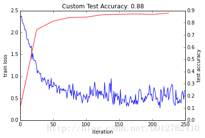
ax2.set_ylabel('test accuracy')
ax2.set_title('Custom Test Accuracy: {:.2f}'.format(test_acc[-1]))

输出9：

Iteration 0 testing...
Iteration 25 testing...
Iteration 50 testing...
Iteration 75 testing...
Iteration 100 testing...
Iteration 125 testing...
Iteration 150 testing...
Iteration 175 testing...
Iteration 200 testing...
Iteration 225 testing...

<matplotlib.text.Text at 0x7f5199af9f50>