A Quick Introduction to Neural Networks

A Quick Introduction to Neural Networks

Posted on
August 9, 2016August 10, 2016 by
ujjwalkarn

An Artificial Neural Network (ANN) is a computational model that is inspired by the way biological neural networks in the human brain process information. Artificial Neural Networks have generated a lot of excitement in Machine
Learning research and industry, thanks to many breakthrough results in speech recognition, computer vision and text processing. In this blog post we will try to develop an understanding of a particular type of Artificial Neural Network called the Multi Layer
Perceptron.

A Single Neuron

The basic unit of computation in a neural network is the
neuron, often called a node or unit. It receives input from some other nodes, or from an external source and computes an output. Each input has an associated
weight (w), which is assigned on the basis of its relative importance to other inputs. The node applies a function f
(defined below) to the weighted sum of its inputs as shown in Figure 1 below:



Figure 1: a single neuron
The above network takes numerical inputs X1 and
X2 and has weights w1 and w2 associated with those inputs. Additionally, there is another input
1 with weight b (called the Bias) associated with it. We will learn more details about role of the bias later.
The output Y from the neuron is computed as shown in the Figure 1. The function
f is non-linear and is called the Activation Function. The purpose of the activation function is to introduce non-linearity into the output of a neuron. This is important because most real world data is non linear and
we want neurons to learn these non linear representations.
Every activation function (or non-linearity) takes a single number and performs a certain fixed mathematical operation on it
[2]. There are several activation functions you may encounter in practice:
Sigmoid: takes a real-valued input and squashes it to range between 0 and 1
σ(x) = 1 / (1 + exp(−x))
tanh: takes a real-valued input and squashes it to the range [-1, 1]
tanh(x) = 2σ(2x) − 1
ReLU: ReLU stands for Rectified Linear Unit. It takes a real-valued input and thresholds it at zero (replaces negative values with zero)
f(x) = max(0, x)
The below figures [2]  show each of the above activation functions.



Figure 2: different activation functions
Importance of Bias: The main function of Bias is to provide every node with a trainable constant value (in addition to the normal inputs that the node receives). See

this link to learn more about the role of bias in a neuron.

Feedforward Neural Network

The feedforward neural network was the first and simplest type of artificial neural network devised
[3]. It contains multiple neurons (nodes) arranged in
layers. Nodes from adjacent layers have connections or
edges between them. All these connections have weights associated with them.
An example of a feedforward neural network is shown in Figure 3.



Figure 3: an example of feedforward neural network
A feedforward neural network can consist of three types of nodes:
Input Nodes – The Input nodes provide information from the outside world to the network and are together referred to as the “Input Layer”. No computation is performed in any of the Input nodes – they just pass on the information to the
hidden nodes.
Hidden Nodes – The Hidden nodes have no direct connection with the outside world (hence the name “hidden”). They perform computations and transfer information from the input nodes to the output nodes. A collection of hidden nodes forms
a “Hidden Layer”. While a feedforward network will only have a single input layer and a single output layer, it can have zero or multiple Hidden Layers.
Output Nodes – The Output nodes are collectively referred to as the “Output Layer” and are responsible for computations and transferring information from the network to the outside world.
In a feedforward network, the information moves in only one direction – forward – from the input nodes, through the hidden nodes (if any) and to the output nodes. There are no cycles or loops in the network
[3] (this property of feed forward networks is different from Recurrent Neural Networks in which the connections between the nodes form a cycle).
Two examples of feedforward networks are given below:

Single Layer Perceptron – This is the simplest feedforward neural network
[4] and does not contain any hidden layer. You can learn more about Single Layer Perceptrons in
[4], [5],
[6], [7].

Multi Layer Perceptron – A Multi Layer Perceptron has one or more hidden layers. We will only discuss Multi Layer Perceptrons below since they are more useful than Single Layer Perceptons for practical applications
today.

Multi Layer Perceptron

A Multi Layer Perceptron (MLP) contains one or more hidden layers (apart from one input and one output layer).  While a single layer perceptron can only learn linear functions, a multi layer perceptron can also learn non – linear
functions.
Figure 4 shows a multi layer perceptron with a single hidden layer. Note that all connections have weights associated with them, but only three weights (w0, w1, w2) are shown in the figure.
Input Layer: The Input layer has three nodes. The Bias node has a value of 1. The other two nodes take X1 and X2 as external inputs (which are numerical values depending upon the input dataset). As discussed above,
no computation is performed in the Input layer, so the outputs from nodes in the Input layer are 1, X1 and X2 respectively, which are fed into the Hidden Layer.
Hidden Layer: The Hidden layer also has three nodes with the Bias node having an output of 1. The output of the other two nodes in the Hidden layer depends on the outputs from the Input layer (1, X1, X2) as well
as the weights associated with the connections (edges). Figure 4 shows the output calculation for one of the hidden nodes (highlighted). Similarly, the output from other hidden node can be calculated. Remember that f
refers to the activation function. These outputs are then fed to the nodes in the Output layer.



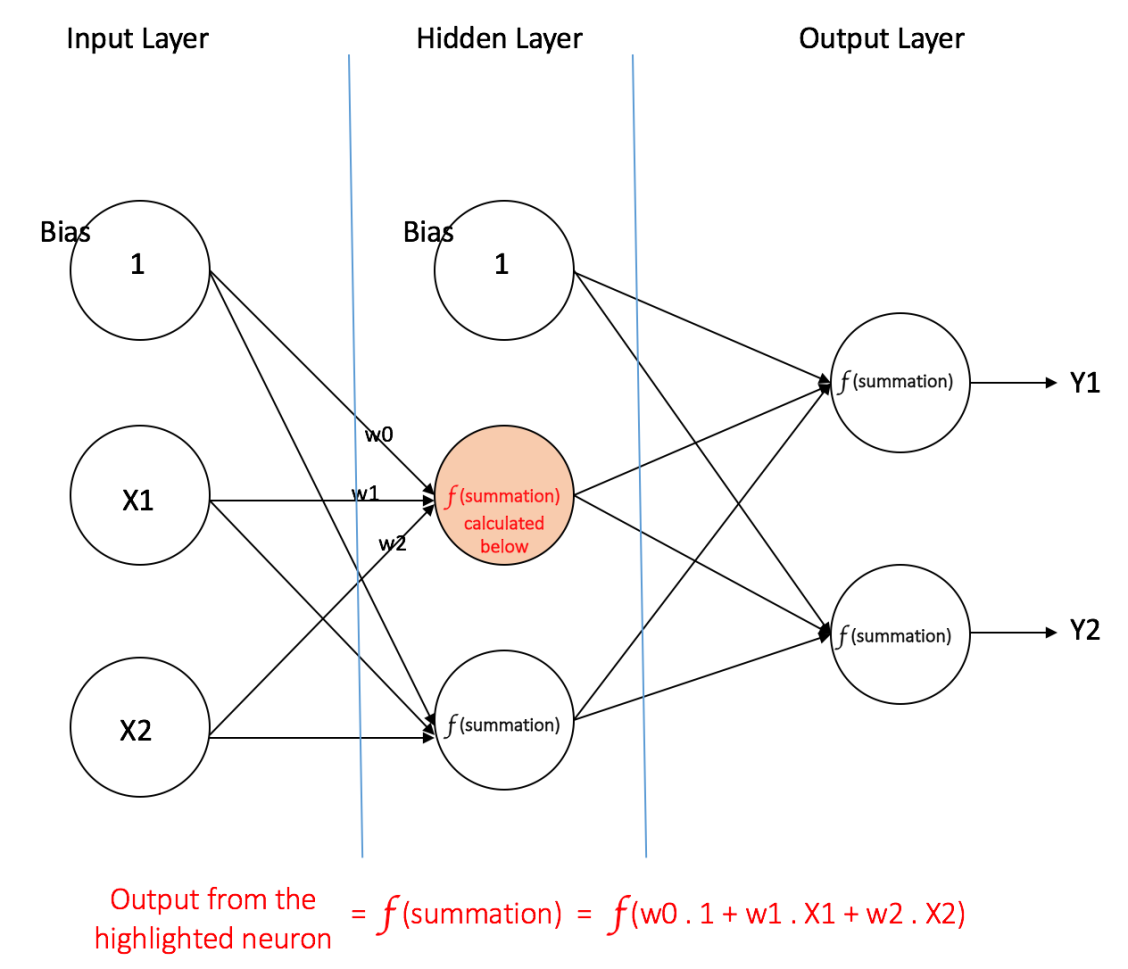
Figure 4: a multi layer perceptron having one hidden layer
Output Layer: The Output layer has two nodes which take inputs from the Hidden layer and perform similar computations as shown for the highlighted hidden node. The values calculated (Y1 and Y2) as a result of these
computations act as outputs of the Multi Layer Perceptron.
Given a set of features X = (x1, x2, …) and a target
y, a Multi Layer Perceptron can learn the relationship between the features and the target, for either classification or regression.
Lets take an example to understand Multi Layer Perceptrons better. Suppose we have the following student-marks dataset:



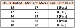
The two input columns show the number of hours the student has studied and the mid term marks obtained by the student. The Final Result column can have two values 1 or 0 indicating whether the student passed in the final term. For
example, we can see that if the student studied 35 hours and had obtained 67 marks in the mid term, he / she ended up passing the final term.
Now, suppose, we want to predict whether a student studying 25 hours and having 70 marks in the mid term will pass the final term.



This is a binary classification problem where a multi layer perceptron can learn from the given examples (training data) and make an informed prediction given a new data point. We will see below how a multi layer perceptron learns
such relationships.
Training our MLP: The Back-Propagation Algorithm
The process by which a Multi Layer Perceptron learns is called the Backpropagation algorithm. I would recommend reading

this Quora answer by Hemanth Kumar (quoted below) which explains Backpropagation clearly.

Backward Propagation of Errors, often abbreviated as BackProp is one of the several ways in which an artificial neural network (ANN) can be trained. It is a supervised training scheme, which means, it learns from
labeled training data (there is a supervisor, to guide its learning).
To put in simple terms, BackProp is like “learning from mistakes“. The supervisor corrects the ANN whenever it makes mistakes.
An ANN consists of nodes in different layers; input layer, intermediate hidden layer(s) and the output layer. The connections between nodes of adjacent layers have “weights” associated with them. The goal of learning is to assign
correct weights for these edges. Given an input vector, these weights determine what the output vector is.
In supervised learning, the training set is labeled. This means, for some given inputs, we know the desired/expected output (label).
BackProp Algorithm:

Initially all the edge weights are randomly assigned. For every input in the training dataset, the ANN is activated and its output is observed. This output is compared with the desired output that we already know, and the error is “propagated” back to the previous
layer. This error is noted and the weights are “adjusted” accordingly. This process is repeated until the output error is below a predetermined threshold.
Once the above algorithm terminates, we have a “learned” ANN which, we consider is ready to work with “new” inputs. This ANN is said to have learned from several examples (labeled data) and from its mistakes (error propagation).

Now that we have an idea of how Backpropagation works, lets come back to our student-marks dataset shown above.
The Multi Layer Perceptron shown in Figure 5 (adapted from Sebastian Raschka’s excellent
visual explanation of the backpropagation algorithm) has two nodes in the input layer (apart from the Bias node) which take the inputs ‘Hours Studied’ and ‘Mid Term Marks’. It also has a hidden layer with two nodes (apart from the Bias node). The output
layer has two nodes as well – the upper node outputs the probability of ‘Pass’ while the lower node outputs the probability of ‘Fail’.
In classification tasks, we generally use a
Softmax function as the Activation Function in the Output layer of the Multi Layer Perceptron to ensure that the outputs are probabilities and they add up to 1. The Softmax function takes a vector of arbitrary real-valued scores and squashes it to a vector
of values between zero and one that sum to one. So, in this case,
Probability (Pass) + Probability (Fail) = 1
Step 1: Forward Propagation
All weights in the network are randomly assigned. Lets consider the hidden layer node marked
V in Figure 5 below. Assume the weights of the connections from the inputs to that node are w1, w2 and w3 (as shown).
The network then takes the first training example as input (we know that for inputs 35 and 67, the probability of Pass is 1).
Input to the network = [35, 67]
Desired output from the network (target) = [1, 0]
Then output V from the node in consideration can be calculated as below ([b]f
[/b]is an activation function such as sigmoid):
V = f (1*w1 + 35*w2 + 67*w3)
Similarly, outputs from the other node in the hidden layer is also calculated. The outputs of the two nodes in the hidden layer act as inputs to the two nodes in the output layer. This enables us to calculate output probabilities
from the two nodes in output layer.
Suppose the output probabilities from the two nodes in the output layer are 0.4 and 0.6 respectively (since the weights are randomly assigned, outputs will also be random). We can see that the calculated probabilities (0.4 and
0.6) are very far from the desired probabilities (1 and 0 respectively), hence the network in Figure 5 is said to have an ‘Incorrect Output’.



Figure 5: forward propagation step in a multi layer perceptron
Step 2: Back Propagation and Weight Updation
We calculate the total error at the output nodes and propagate these errors back through the network using Backpropagation to calculate the
gradients. Then we use an optimization method such as Gradient Descent to ‘adjust’ all weights in the network with an aim of reducing the error at the output layer. This is shown in the Figure 6 below (ignore the mathematical
equations in the figure for now).
Suppose that the new weights associated with the node in consideration are w4, w5 and w6 (after Backpropagation and adjusting weights).



Figure 6: backward propagation and weight updation step in a multi layer perceptron
If we now input the same example to the network again, the network should perform better than before since the weights have now been adjusted to minimize the error in prediction. As shown in Figure 7, the errors at the output nodes now
reduce to [0.2, -0.2] as compared to [0.6, -0.4] earlier. This means that our network has learnt to correctly classify our first training example.



Figure 7: the MLP network now performs better on the same input
We repeat this process with all other training examples in our dataset. Then, our network is said to have
learnt those examples.
If we now want to predict whether a student studying 25 hours and having 70 marks in the mid term will pass the final term, we go through the forward propagation step and find the output probabilities for Pass and Fail.
I have avoided mathematical equations and explanation of concepts such as ‘Gradient Descent’ here and have rather tried to develop an intuition for the algorithm. For a more mathematically involved discussion of the Backpropagation
algorithm, refer to this link.

3d Visualization of a Multi Layer Perceptron

Adam Harley has created a 3d visualization of a Multi Layer Perceptron which has already been trained (using Backpropagation) on the MNIST Database
of handwritten digits.
The network takes 784 numeric pixel values as inputs from a 28 x 28 image of a handwritten digit (it has 784 nodes in the Input Layer corresponding to pixels). The network has 300 nodes in the first hidden layer, 100 nodes in the
second hidden layer, and 10 nodes in the output layer (corresponding to the 10 digits)
[15].
Although the network described here is much larger (uses more hidden layers and nodes) compared to the one we discussed in the previous section, all computations in the forward propagation step and backpropagation step are done
in the same way (at each node) as discussed before.
Figure 8 shows the network when the input is the digit ‘5’.



Figure 8: visualizing the network for an input of ‘5’
A node which has a higher output value than others is represented by a brighter color. In the Input layer, the bright nodes are those which receive higher numerical pixel values as input. Notice how in the output layer, the only
bright node corresponds to the digit 5 (it has an output probability of 1, which is higher than the other nine nodes which have an output probability of 0). This indicates that the MLP has correctly classified the input digit. I highly recommend playing around
with this visualization and observing connections between nodes of different layers.

Deep Neural Networks

What is the difference between deep learning and usual machine learning?
What is the difference between a neural network and a deep neural network?
How is deep learning different from multilayer perceptron?

Conclusion

I have skipped important details of some of the concepts discussed in this post to facilitate understanding. I would recommend going through

Part1,
Part2,
Part3 and
Case Study from Stanford’s Neural Network tutorial for a thorough understanding of Multi Layer Perceptrons.
Let me know in the comments below if you have any questions or suggestions!

References

Artificial Neuron Models
Neural Networks Part 1: Setting up the Architecture (Stanford CNN Tutorial)
Wikipedia article on Feed Forward Neural Network
Wikipedia article on Perceptron 
Single-layer Neural Networks (Perceptrons) 
Single Layer Perceptrons 
Weighted Networks – The Perceptron
Neural network models (supervised) (scikit learn documentation)
What does the hidden layer in a neural network compute?
How to choose the number of hidden layers and nodes in a feedforward neural network? 
Crash Introduction to Artificial Neural Networks
Why the BIAS is necessary in ANN? Should we have separate BIAS for
each layer?
Basic Neural Network Tutorial – Theory
Neural Networks Demystified (Video Series): Part 1, Welch Labs @ MLconf SF
A. W. Harley, “An Interactive Node-Link Visualization of Convolutional Neural Networks,” in ISVC, pages 867-877, 2015 (link)

Share this:

Tweet

inShare94

Related

An
Intuitive Explanation of Convolutional Neural NetworksIn "Deep Learning"
Curated
list of Python tutorials for Data ScienceIn "Python"
Introducing
xda: R package for exploratory data analysisIn "R Language"

Posted in

Deep Learning