Image Completion with Deep Learning in TensorFlow【DCGAN,图像补全】
2017-09-13 09:36
916 查看
写的不错,直接拿来了。
http://bamos.github.io/2016/08/09/deep-completion/#so-how-can-we-complete-images
Introduction
Step 1: Interpreting images as samples
from a probability distribution
How would you fill in the missing information?
But where does statistics fit in? These are images.
So how can we complete images?
Step 2: Quickly generating fake images
Learning to generate new samples
from an unknown probability distribution
[ML-Heavy] Generative Adversarial Net (GAN) building
blocks
Using G(z)G(z) to
produce fake images
[ML-Heavy] Training DCGANs
Existing GAN and DCGAN implementations
[ML-Heavy] DCGANs in TensorFlow
Running DCGAN on your images
Step 3: Finding the best fake image for image completion
Image completion with DCGANs
[ML-Heavy] Loss function for projecting onto pgpg
[ML-Heavy] TensorFlow implementation of
image completion with DCGANs
Completing your images
Conclusion
Citation for this article/project
Partial bibliography for further reading
Bonus: Incomplete Thoughts on TensorFlow and Torch
Content-aware fill is a powerful tool designers and photographers use to fill in unwanted or missing parts of images. Image completion and inpainting are
closely related technologies used to fill in missing or corrupted parts of images. There are many ways to do content-aware fill, image completion, and inpainting. In this blog post, I present Raymond Yeh and Chen Chen et al.’s paper “Semantic
Image Inpainting with Perceptual and Contextual Losses,” which was just posted on arXiv on July 26, 2016. This paper shows how to use deep learning for image completion with a DCGAN.
This blog post is meant for a general technical audience with some deeper portions for people with a machine learning background. I’ve added
to sections to indicate that the section can be skipped if you don’t want too many details. We will only look at the constrained case of completing missing pixels from images of faces. I have released all of the TensorFlow source
code behind this post on GitHub at bamos/dcgan-completion.tensorflow.
We’ll approach image completion in three steps.
We’ll first interpret images as being
samples from a probability distribution.
This interpretation lets us learn how to generate fake images.
Then we’ll find the best fake image for completion.
Photoshop example of automatically filling in missing image parts. (Image CC licensed, source.)
Photoshop example of automatically removing unwanted image parts. (Image CC licensed, source.)
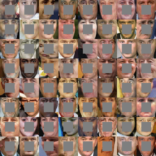
Completions generated by what we’ll cover in this blog post. The centers of these images are being automatically generated. The source code to create this is available here. These
are not curated! I selected a random subset of images from the LFW dataset.
In the examples above, imagine you’re building a system to fill in the missing pieces. How would you do it? How do you think the human brain does it? What kind of information would you use?
In this post we will focus on two types of information:
Contextual information: You can infer what missing pixels are based on information provided by surrounding pixels.
Perceptual information: You interpret the filled in portions as being “normal,” like from what you’ve seen in real life or from other pictures.
Both of these are important. Without contextual information, how do you know what to fill in? Without perceptual information, there are many valid completions for a context. Something that looks “normal” to a machine learning system might not look normal to
humans.
It would be nice to have an exact, intuitive algorithm that captures both of these properties that says step-by-step how to complete an image. Creating such an algorithm may be possible for specific cases, but in general, nobody knows how. Today’s best approaches
use statistics and machine learning to learn an approximate technique.
To motivate the problem, let’s start by looking at a probability distribution that is well-understood and can be
represented concisely in closed form: a normal distribution. Here’s the probability
density function (PDF) for a normal distribution. You can interpret the PDF as going over the input space horizontally with the vertical axis showing the probability that some value occurs. (If you’re interested, the code to create
these plots is available at bamos/dcgan-completion.tensorflow:simple-distributions.py.)
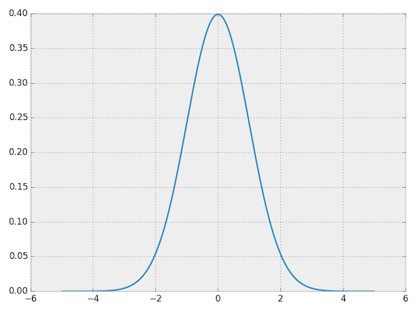
PDF for a normal distribution.
Let’s sample from the distribution to get some data. Make sure you understand the connection between the PDF and the samples.
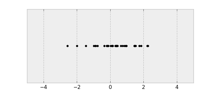
Samples from a normal distribution.
This is a 1D probability distribution because the input only goes along a single dimension. We can do the same thing in two dimensions.
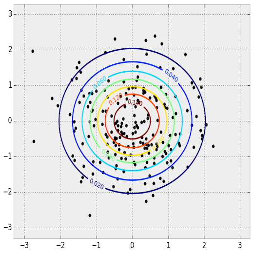
PDF and samples from a 2D normal distribution. The PDF is shown as a contour plot and the samples are overlaid.
The key relationship between images and statistics is that we can interpret images as samples from a high-dimensional probability distribution. The probability distribution goes over the pixels of images. Imagine you’re taking a picture
with your camera. This picture will have some finite number of pixels. When you take an image with your camera, you are sampling from this complex probability distribution. This distribution is what we’ll use to define what makes an image normal or not. With
images, unlike with the normal distributions, we don’t know the true probability distribution and we can only collect samples.
In this post, we’ll use color images represented by the RGB color model. Our images will be 64 pixels wide and 64 pixels
high, so our probability distribution has 64⋅64⋅3≈12k64⋅64⋅3≈12k dimensions.
Let’s first consider the multivariate normal distribution from before for intuition. Given x=1x=1,
what is the most probable yy value?
We can find this by maximizing the value of the PDF over all possible yy values
with x=1x=1 fixed.
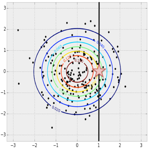
Finding the most probable yy value
given some fixed xx in
a multivariate normal distribution.
This concept naturally extends to our image probability distribution when we know some values and want to complete the missing values. Just pose it as a maximization problem where we search over all of the possible missing values. The completion will be the
most probable image.
Visually looking at the samples from the normal distribution, it seems reasonable that we could find the PDF given only samples. Just pick your favorite statistical
model and fit it to the data.
However we don’t use this method in practice. While the PDF is easy to recover for simple distributions, it’s difficult and often intractable for more complex distributions over images. The complexity partly comes from intricate conditional
dependencies: the value of one pixel depends on the values of other pixels in the image. Also, maximizing over a general PDF is an extremely difficult and often intractable non-convex optimization problem.
Instead of learning how to compute the PDF, another well-studied idea in statistics is to learn how to generate new (random) samples with a generative
model. Generative models can often be difficult to train or intractable, but lately the deep learning community has made some amazing progress in this space. Yann
LeCun gives a great introduction to one way of training generative models (adversarial training) in this
Quora post, describing the idea as the most interesting idea in the last 10 years in machine learning:
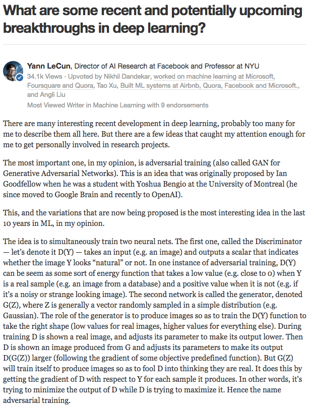
Yann LeCun’s introduction to adversarial training from this
Quora post.

Street Fighter analogy for adversarial networks from the EyeScream post. The networks fight each other and improve together, like two humans
playing against each other in a game.Image source.
There are other ways to train generative models with deep learning, like Variational Autoencoders (VAEs). In this post we’ll only focus
on Generative Adversarial Nets (GANs).
These ideas started with Ian Goodfellow et al.’s landmark paper “Generative Adversarial Nets” (GANs), published
at the Neural Information Processing Systems (NIPS) conference in 2014. The idea is that we define a simple, well-known distribution and represent it
as pzpz.
For the rest of this post, we’ll use pzpz as
a uniform distribution between -1 and 1 (inclusively). We represent sampling a number from this distribution as z∼pzz∼pz.
If pzpz is
5-dimensional, we can sample it with one line of Python with numpy:
Now this we have a simple distribution we can easily sample from, we’d like to define a function G(z)G(z) that
produces samples from our original probability distribution.
So how do we define G(z)G(z) so
that it takes a vector on input and returns an image? We’ll use a deep neural network. There are many great introductions to deep neural network basics, so I won’t cover them here. Some great references that I recommend are Stanford’s
CS231n course, Ian Goodfellow et al.’s Deep Learning Book, Image
Kernels Explained Visually, and convolution arithmetic guide.
There are many ways we can structure G(z)G(z) with
deep learning. The original GAN paper proposed the idea, a training procedure, and preliminary experimental results. The idea has been greatly built on and improved. One of the most recent ideas was presented in the paper “Unsupervised
Representation Learning with Deep Convolutional Generative Adversarial Networks” by Alec Radford, Luke Metz, and Soumith Chintala at the International
Conference on Learning Representations (ICLR, pronounced “eye-clear”) in 2016. This paper presents deep convolutional GANs (called DCGANs) that use fractionally-strided convolutions to upsample images.
What is a fractionally-strided convolution and how do they upsample images? Vincent Dumoulin and Francesco Visin’s paper “A
guide to convolution arithmetic for deep learning” and conv_arithmetic project is a very well-written introduction to
convolution arithmetic in deep learning. The visualizations are amazing and give great intuition into how fractionally-strided convolutions work. First, make sure you understand how a normal convolution slides a kernel over a (blue) input space to produce
the (green) output space. Here, the output is smaller than the input. (If you don’t, go through the CS231n CNN section or
the convolution arithmetic guide.)
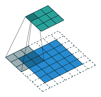
Illustration of a convolution from the input (blue) to output (green). This image is from vdumoulin/conv_arithmetic.
Next, suppose that you have a 3x3 input. Our goal is to upsample so that the output is larger. You can interpret a fractionally-strided convolution as expanding the pixels so that there are zeros in-between the pixels. Then the convolution over this expanded
space will result in a larger output space. Here, it’s 5x5.
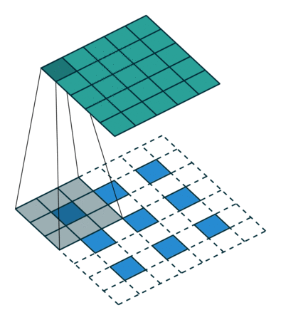
Illustration of a fractionally-strided convolution from the input (blue) to output (green). This image is from vdumoulin/conv_arithmetic.
As a side-note, there are many names for convolutional layers that upsample: full convolution, in-network
upsampling, fractionally-strided convolution, backwards convolution, deconvolution, upconvolution, or transposed convolution. Using the term ‘deconvolution’ for this is strongly discouraged because it’s an over-loaded term: the
mathematical operation or other uses in computer vision have a completely different meaning.
Now that we have fractionally-strided convolutions as building blocks, we can finally represent G(z)G(z) so
that it takes a vector z∼pzz∼pzon
input and outputs a 64x64x3 RGB image.
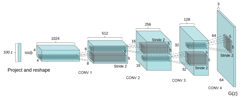
One way to structure the generator G(z)G(z) with
a DCGAN. This image is from the DCGAN paper.
The DCGAN paper also presents other tricks and modifications for training DCGANs like using batch normalization or leaky ReLUs if you’re
interested.
Let’s pause and appreciate how powerful this formulation of G(z)G(z) is.
The DCGAN paper showed how a DCGAN can be trained on a dataset of bedroom images. Then sampling G(z)G(z) will
produce the following fake images of what the generator thinks bedrooms looks like. None of these images are in the original dataset!
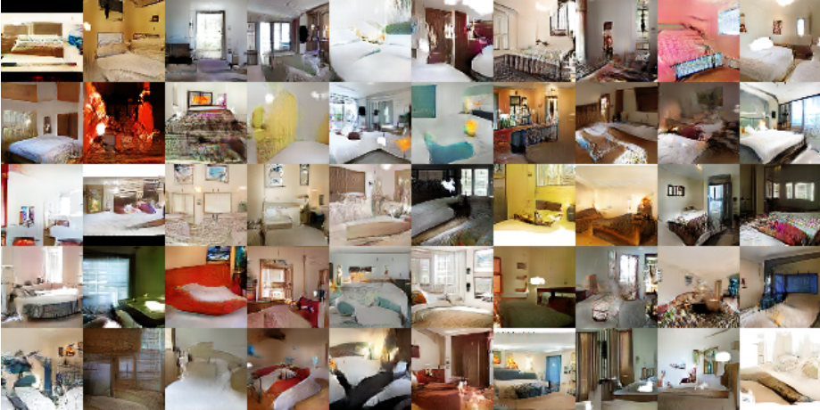
Generating bedroom images with a DCGAN. This image is from the DCGAN paper.
Also, you can perform vector arithmetic on the zz input
space. The following is on a network trained to produce faces.
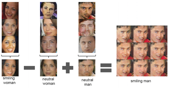
Face arithmetic with DCGANs. This image is from the DCGAN paper.
Now that we have defined G(z)G(z) and
have seen how powerful the formulation is, how do we train it? We have a lot of latent variables(or parameters) that we
need to find. This is where using adversarial networks comes in.
First let’s define some notation. Let the (unknown) probability distribution of our data be pdatapdata.
Also we can interpret G(z)G(z) (where z∼pzz∼pz)
as drawing samples from a probability distribution, let’s call it the generative probability distribution, pgpg.
The discriminator network D(x)D(x) takes
some image xx on
input and returns the probability that the image xx was
sampled from pdatapdata.
The discriminator should return a value closer to 1 when the image is from pdatapdata and
a value closer to 0 when the image is fake, like an image sampled from pgpg.
In DCGANs, D(x)D(x) is
a traditional convolutional network.
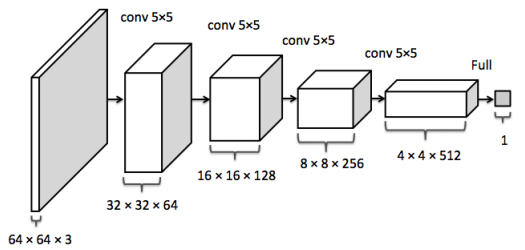
The discriminator convolutional network. This image is from the inpainting paper.
The goal of training the discriminator D(x)D(x) is:
Maximize D(x)D(x) for
every image from the true data distribution x∼pdatax∼pdata.
Minimize D(x)D(x) for
every image not from the true data distribution x≁pdatax≁pdata.
The goal of training the generator G(z)G(z) is
to produce samples that fool DD.
The output of the generator is an image and can be used as the input to the discriminator. Therefore, the generator wants to to maximize D(G(z))D(G(z)),
or equivalently minimize 1−D(G(z))1−D(G(z))because DD is
a probability estimate and only ranges between 0 and 1.
As presented in the paper, training adversarial networks is done with the following minimax game. The expectations in
the first term go over the samples from the true data distribution and over samples from pzpz in
the second term, which goes over G(z)∼pgG(z)∼pg.
minGmaxDEx∼pdatalogD(x)+Ez∼pz[log(1−D(G(z)))]minGmaxDEx∼pdatalogD(x)+Ez∼pz[log(1−D(G(z)))]
We will train DD and GG by
taking the gradients of this expression with respect to their parameters. We know how to quickly compute every part of this expression. The expectations are approximated in minibatches of size m,m, and
the inner maximization can be approximated with kk gradient
steps. It turns out k=1k=1 works
well for training.
Let θdθd be
the parameters of the discriminator and θgθg be
the parameters the generator. The gradients of the loss with respect to θdθd and θgθg can
be computed with backpropagation because DD and GG are
defined by well-understood neural network components. Here’s the training algorithm from the GAN paper. Ideally
once this is finished, pg=pdatapg=pdata,
so G(z)G(z) will
be able to produce new samples from pdatapdata.
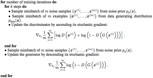
GAN training algorithm from the GAN paper.
There are many great GAN and DCGAN implementations on GitHub you can browse:
goodfeli/adversarial: Theano GAN implementation released by the authors of the GAN paper.
tqchen/mxnet-gan: Unofficial MXNet GAN implementation.
Newmu/dcgan_code: Theano DCGAN implementation released by the authors of the DCGAN paper.
soumith/dcgan.torch: Torch DCGAN implementation by one of the authors (Soumith Chintala) of the DCGAN paper.
carpedm20/DCGAN-tensorflow: Unofficial TensorFlow DCGAN implementation.
openai/improved-gan: Code behind OpenAI’s
first paper. Extensively modifies
mattya/chainer-DCGAN: Unofficial Chainer DCGAN implementation.
jacobgil/keras-dcgan: Unofficial (and incomplete) Keras DCGAN implementation.
Moving forward, we will build on carpedm20/DCGAN-tensorflow.
The implementation for this portion is in my bamos/dcgan-completion.tensorflow GitHub repository. I strongly emphasize
that the code in this portion is from Taehoon Kim’s carpedm20/DCGAN-tensorflow repository. We’ll use my repository here
so that we can easily use the image completion portions in the next section.
The implementation is mostly in a Python class called
It’s helpful to have everything in a class like this so that intermediate states can be saved after training and then loaded for later use.
First let’s define the generator and discriminator architectures. The
and
When we’re initializing this class, we’ll use these functions to create the models. We need two versions of the discriminator that shares (or reuses) parameters. One for the minibatch of images from the data distribution and the other for the minibatch of images
from the generator.
Next, we’ll define the loss functions. Instead of using the sums, we’ll use the cross entropy between DD’s
predictions and what we want them to be because it works better. The discriminator wants the predictions on the “real” data to be all ones and the predictions on the “fake” data from the generator to be all zeros. The generator wants the discriminator’s predictions
to be all ones.
Gather the variables for each of the models so they can be trained separately.
Now we’re ready to optimize the parameters and we’ll use ADAM, which is an adaptive non-convex optimization method commonly used in modern
deep learning. ADAM is often competitive with SGD and (usually) doesn’t require hand-tuning of the learning rate, momentum, and other hyper-parameters.
We’re ready to go through our data. In each epoch, we sample some images in a minibatch and run the optimizers to update the networks. Interestingly if GG is
only updated once, the discriminator’s loss does not go to zero. Also, I think the additional calls at the end to
causing a little bit of unnecessary computation and are redundant because these values are computed as part of
As an exercise in TensorFlow, you can try optimizing this part and send a PR to the original repo. (If you do, ping me and I’ll update it in mine too.)
That’s it! Of course the full code has a little more book-keeping that you can check out in model.py.
If you skipped the last section, but are interested in running some code: The implementation for this portion is in my bamos/dcgan-completion.tensorflow GitHub
repository. I strongly emphasize that the code in this portion is from Taehoon Kim’scarpedm20/DCGAN-tensorflow repository.
We’ll use my repository here so that we can easily use the image completion portions in the next section. As a warning, if you don’t have a CUDA-enabled GPU, training the network in this portion may be prohibitively slow.
Please message me if the following doesn’t work for you!
First let’s clone my bamos/dcgan-completion.tensorflow and OpenFace repositories.
We’ll use OpenFace’s Python-only portions to pre-process images. Don’t worry, you won’t have to install OpenFace’s Torch dependency. Create a new working directory for this and clone the repositories:
http://bamos.github.io/2016/08/09/deep-completion/#so-how-can-we-complete-images
Introduction
Step 1: Interpreting images as samples
from a probability distribution
How would you fill in the missing information?
But where does statistics fit in? These are images.
So how can we complete images?
Step 2: Quickly generating fake images
Learning to generate new samples
from an unknown probability distribution
[ML-Heavy] Generative Adversarial Net (GAN) building
blocks
Using G(z)G(z) to
produce fake images
[ML-Heavy] Training DCGANs
Existing GAN and DCGAN implementations
[ML-Heavy] DCGANs in TensorFlow
Running DCGAN on your images
Step 3: Finding the best fake image for image completion
Image completion with DCGANs
[ML-Heavy] Loss function for projecting onto pgpg
[ML-Heavy] TensorFlow implementation of
image completion with DCGANs
Completing your images
Conclusion
Citation for this article/project
Partial bibliography for further reading
Bonus: Incomplete Thoughts on TensorFlow and Torch
Introduction
Content-aware fill is a powerful tool designers and photographers use to fill in unwanted or missing parts of images. Image completion and inpainting areclosely related technologies used to fill in missing or corrupted parts of images. There are many ways to do content-aware fill, image completion, and inpainting. In this blog post, I present Raymond Yeh and Chen Chen et al.’s paper “Semantic
Image Inpainting with Perceptual and Contextual Losses,” which was just posted on arXiv on July 26, 2016. This paper shows how to use deep learning for image completion with a DCGAN.
This blog post is meant for a general technical audience with some deeper portions for people with a machine learning background. I’ve added
[ML-Heavy]tags
to sections to indicate that the section can be skipped if you don’t want too many details. We will only look at the constrained case of completing missing pixels from images of faces. I have released all of the TensorFlow source
code behind this post on GitHub at bamos/dcgan-completion.tensorflow.
We’ll approach image completion in three steps.
We’ll first interpret images as being
samples from a probability distribution.
This interpretation lets us learn how to generate fake images.
Then we’ll find the best fake image for completion.
Photoshop example of automatically filling in missing image parts. (Image CC licensed, source.)
Photoshop example of automatically removing unwanted image parts. (Image CC licensed, source.)
Completions generated by what we’ll cover in this blog post. The centers of these images are being automatically generated. The source code to create this is available here. These
are not curated! I selected a random subset of images from the LFW dataset.
Step 1: Interpreting images as samples from a probability distribution
How would you fill in the missing information?
In the examples above, imagine you’re building a system to fill in the missing pieces. How would you do it? How do you think the human brain does it? What kind of information would you use?In this post we will focus on two types of information:
Contextual information: You can infer what missing pixels are based on information provided by surrounding pixels.
Perceptual information: You interpret the filled in portions as being “normal,” like from what you’ve seen in real life or from other pictures.
Both of these are important. Without contextual information, how do you know what to fill in? Without perceptual information, there are many valid completions for a context. Something that looks “normal” to a machine learning system might not look normal to
humans.
It would be nice to have an exact, intuitive algorithm that captures both of these properties that says step-by-step how to complete an image. Creating such an algorithm may be possible for specific cases, but in general, nobody knows how. Today’s best approaches
use statistics and machine learning to learn an approximate technique.
But where does statistics fit in? These are images.
To motivate the problem, let’s start by looking at a probability distribution that is well-understood and can berepresented concisely in closed form: a normal distribution. Here’s the probability
density function (PDF) for a normal distribution. You can interpret the PDF as going over the input space horizontally with the vertical axis showing the probability that some value occurs. (If you’re interested, the code to create
these plots is available at bamos/dcgan-completion.tensorflow:simple-distributions.py.)
PDF for a normal distribution.
Let’s sample from the distribution to get some data. Make sure you understand the connection between the PDF and the samples.
Samples from a normal distribution.
This is a 1D probability distribution because the input only goes along a single dimension. We can do the same thing in two dimensions.
PDF and samples from a 2D normal distribution. The PDF is shown as a contour plot and the samples are overlaid.
The key relationship between images and statistics is that we can interpret images as samples from a high-dimensional probability distribution. The probability distribution goes over the pixels of images. Imagine you’re taking a picture
with your camera. This picture will have some finite number of pixels. When you take an image with your camera, you are sampling from this complex probability distribution. This distribution is what we’ll use to define what makes an image normal or not. With
images, unlike with the normal distributions, we don’t know the true probability distribution and we can only collect samples.
In this post, we’ll use color images represented by the RGB color model. Our images will be 64 pixels wide and 64 pixels
high, so our probability distribution has 64⋅64⋅3≈12k64⋅64⋅3≈12k dimensions.
So how can we complete images?
Let’s first consider the multivariate normal distribution from before for intuition. Given x=1x=1,what is the most probable yy value?
We can find this by maximizing the value of the PDF over all possible yy values
with x=1x=1 fixed.
Finding the most probable yy value
given some fixed xx in
a multivariate normal distribution.
This concept naturally extends to our image probability distribution when we know some values and want to complete the missing values. Just pose it as a maximization problem where we search over all of the possible missing values. The completion will be the
most probable image.
Visually looking at the samples from the normal distribution, it seems reasonable that we could find the PDF given only samples. Just pick your favorite statistical
model and fit it to the data.
However we don’t use this method in practice. While the PDF is easy to recover for simple distributions, it’s difficult and often intractable for more complex distributions over images. The complexity partly comes from intricate conditional
dependencies: the value of one pixel depends on the values of other pixels in the image. Also, maximizing over a general PDF is an extremely difficult and often intractable non-convex optimization problem.
Step 2: Quickly generating fake images
Learning to generate new samples from an unknown probability distribution
Instead of learning how to compute the PDF, another well-studied idea in statistics is to learn how to generate new (random) samples with a generativemodel. Generative models can often be difficult to train or intractable, but lately the deep learning community has made some amazing progress in this space. Yann
LeCun gives a great introduction to one way of training generative models (adversarial training) in this
Quora post, describing the idea as the most interesting idea in the last 10 years in machine learning:
Yann LeCun’s introduction to adversarial training from this
Quora post.
Street Fighter analogy for adversarial networks from the EyeScream post. The networks fight each other and improve together, like two humans
playing against each other in a game.Image source.
There are other ways to train generative models with deep learning, like Variational Autoencoders (VAEs). In this post we’ll only focus
on Generative Adversarial Nets (GANs).
[ML-Heavy] Generative Adversarial Net (GAN) building blocks
These ideas started with Ian Goodfellow et al.’s landmark paper “Generative Adversarial Nets” (GANs), publishedat the Neural Information Processing Systems (NIPS) conference in 2014. The idea is that we define a simple, well-known distribution and represent it
as pzpz.
For the rest of this post, we’ll use pzpz as
a uniform distribution between -1 and 1 (inclusively). We represent sampling a number from this distribution as z∼pzz∼pz.
If pzpz is
5-dimensional, we can sample it with one line of Python with numpy:
z = np.random.uniform(-1, 1, 5)
array([ 0.77356483,  0.95258473, -0.18345086,  0.69224724, -0.34718733])
Now this we have a simple distribution we can easily sample from, we’d like to define a function G(z)G(z) that
produces samples from our original probability distribution.
def G(z):
...
return imageSample

z = np.random.uniform(-1, 1, 5)
imageSample = G(z)
So how do we define G(z)G(z) so
that it takes a vector on input and returns an image? We’ll use a deep neural network. There are many great introductions to deep neural network basics, so I won’t cover them here. Some great references that I recommend are Stanford’s
CS231n course, Ian Goodfellow et al.’s Deep Learning Book, Image
Kernels Explained Visually, and convolution arithmetic guide.
There are many ways we can structure G(z)G(z) with
deep learning. The original GAN paper proposed the idea, a training procedure, and preliminary experimental results. The idea has been greatly built on and improved. One of the most recent ideas was presented in the paper “Unsupervised
Representation Learning with Deep Convolutional Generative Adversarial Networks” by Alec Radford, Luke Metz, and Soumith Chintala at the International
Conference on Learning Representations (ICLR, pronounced “eye-clear”) in 2016. This paper presents deep convolutional GANs (called DCGANs) that use fractionally-strided convolutions to upsample images.
What is a fractionally-strided convolution and how do they upsample images? Vincent Dumoulin and Francesco Visin’s paper “A
guide to convolution arithmetic for deep learning” and conv_arithmetic project is a very well-written introduction to
convolution arithmetic in deep learning. The visualizations are amazing and give great intuition into how fractionally-strided convolutions work. First, make sure you understand how a normal convolution slides a kernel over a (blue) input space to produce
the (green) output space. Here, the output is smaller than the input. (If you don’t, go through the CS231n CNN section or
the convolution arithmetic guide.)
Illustration of a convolution from the input (blue) to output (green). This image is from vdumoulin/conv_arithmetic.
Next, suppose that you have a 3x3 input. Our goal is to upsample so that the output is larger. You can interpret a fractionally-strided convolution as expanding the pixels so that there are zeros in-between the pixels. Then the convolution over this expanded
space will result in a larger output space. Here, it’s 5x5.
Illustration of a fractionally-strided convolution from the input (blue) to output (green). This image is from vdumoulin/conv_arithmetic.
As a side-note, there are many names for convolutional layers that upsample: full convolution, in-network
upsampling, fractionally-strided convolution, backwards convolution, deconvolution, upconvolution, or transposed convolution. Using the term ‘deconvolution’ for this is strongly discouraged because it’s an over-loaded term: the
mathematical operation or other uses in computer vision have a completely different meaning.
Now that we have fractionally-strided convolutions as building blocks, we can finally represent G(z)G(z) so
that it takes a vector z∼pzz∼pzon
input and outputs a 64x64x3 RGB image.
One way to structure the generator G(z)G(z) with
a DCGAN. This image is from the DCGAN paper.
The DCGAN paper also presents other tricks and modifications for training DCGANs like using batch normalization or leaky ReLUs if you’re
interested.
Using G(z)G(z) to
produce fake images
Let’s pause and appreciate how powerful this formulation of G(z)G(z) is.The DCGAN paper showed how a DCGAN can be trained on a dataset of bedroom images. Then sampling G(z)G(z) will
produce the following fake images of what the generator thinks bedrooms looks like. None of these images are in the original dataset!
Generating bedroom images with a DCGAN. This image is from the DCGAN paper.
Also, you can perform vector arithmetic on the zz input
space. The following is on a network trained to produce faces.
Face arithmetic with DCGANs. This image is from the DCGAN paper.
[ML-Heavy] Training DCGANs
Now that we have defined G(z)G(z) andhave seen how powerful the formulation is, how do we train it? We have a lot of latent variables(or parameters) that we
need to find. This is where using adversarial networks comes in.
First let’s define some notation. Let the (unknown) probability distribution of our data be pdatapdata.
Also we can interpret G(z)G(z) (where z∼pzz∼pz)
as drawing samples from a probability distribution, let’s call it the generative probability distribution, pgpg.
| Probability Distribution Notation | Meaning |
|---|---|
| pzpz | The (known, simple) distribution zz goes over |
| pdatapdata | The (unknown) distribution over our images. This is where our images are sampled from. |
| pgpg | The generative distribution that the generator GG samples from. We would like for pg=pdatapg=pdata |
some image xx on
input and returns the probability that the image xx was
sampled from pdatapdata.
The discriminator should return a value closer to 1 when the image is from pdatapdata and
a value closer to 0 when the image is fake, like an image sampled from pgpg.
In DCGANs, D(x)D(x) is
a traditional convolutional network.
The discriminator convolutional network. This image is from the inpainting paper.
The goal of training the discriminator D(x)D(x) is:
Maximize D(x)D(x) for
every image from the true data distribution x∼pdatax∼pdata.
Minimize D(x)D(x) for
every image not from the true data distribution x≁pdatax≁pdata.
The goal of training the generator G(z)G(z) is
to produce samples that fool DD.
The output of the generator is an image and can be used as the input to the discriminator. Therefore, the generator wants to to maximize D(G(z))D(G(z)),
or equivalently minimize 1−D(G(z))1−D(G(z))because DD is
a probability estimate and only ranges between 0 and 1.
As presented in the paper, training adversarial networks is done with the following minimax game. The expectations in
the first term go over the samples from the true data distribution and over samples from pzpz in
the second term, which goes over G(z)∼pgG(z)∼pg.
minGmaxDEx∼pdatalogD(x)+Ez∼pz[log(1−D(G(z)))]minGmaxDEx∼pdatalogD(x)+Ez∼pz[log(1−D(G(z)))]
We will train DD and GG by
taking the gradients of this expression with respect to their parameters. We know how to quickly compute every part of this expression. The expectations are approximated in minibatches of size m,m, and
the inner maximization can be approximated with kk gradient
steps. It turns out k=1k=1 works
well for training.
Let θdθd be
the parameters of the discriminator and θgθg be
the parameters the generator. The gradients of the loss with respect to θdθd and θgθg can
be computed with backpropagation because DD and GG are
defined by well-understood neural network components. Here’s the training algorithm from the GAN paper. Ideally
once this is finished, pg=pdatapg=pdata,
so G(z)G(z) will
be able to produce new samples from pdatapdata.
GAN training algorithm from the GAN paper.
Existing GAN and DCGAN implementations
There are many great GAN and DCGAN implementations on GitHub you can browse:goodfeli/adversarial: Theano GAN implementation released by the authors of the GAN paper.
tqchen/mxnet-gan: Unofficial MXNet GAN implementation.
Newmu/dcgan_code: Theano DCGAN implementation released by the authors of the DCGAN paper.
soumith/dcgan.torch: Torch DCGAN implementation by one of the authors (Soumith Chintala) of the DCGAN paper.
carpedm20/DCGAN-tensorflow: Unofficial TensorFlow DCGAN implementation.
openai/improved-gan: Code behind OpenAI’s
first paper. Extensively modifies
carpedm20/DCGAN-tensorflow.
mattya/chainer-DCGAN: Unofficial Chainer DCGAN implementation.
jacobgil/keras-dcgan: Unofficial (and incomplete) Keras DCGAN implementation.
Moving forward, we will build on carpedm20/DCGAN-tensorflow.
[ML-Heavy] DCGANs in TensorFlow
The implementation for this portion is in my bamos/dcgan-completion.tensorflow GitHub repository. I strongly emphasizethat the code in this portion is from Taehoon Kim’s carpedm20/DCGAN-tensorflow repository. We’ll use my repository here
so that we can easily use the image completion portions in the next section.
The implementation is mostly in a Python class called
DCGANin model.py.
It’s helpful to have everything in a class like this so that intermediate states can be saved after training and then loaded for later use.
First let’s define the generator and discriminator architectures. The
linear,
conv2d_transpose,
conv2d,
and
lrelufunctions are defined in ops.py.
def generator(self, z):
self.z_, self.h0_w, self.h0_b = linear(z, self.gf_dim*8*4*4,
'g_h0_lin', with_w=True)

self.h0 = tf.reshape(self.z_, [-1, 4, 4, self.gf_dim * 8])
h0 = tf.nn.relu(self.g_bn0(self.h0))

self.h1, self.h1_w, self.h1_b = conv2d_transpose(h0,
[self.batch_size, 8, 8, self.gf_dim*4], name='g_h1', with_w=True)
h1 = tf.nn.relu(self.g_bn1(self.h1))

h2, self.h2_w, self.h2_b = conv2d_transpose(h1,
[self.batch_size, 16, 16, self.gf_dim*2], name='g_h2', with_w=True)
h2 = tf.nn.relu(self.g_bn2(h2))

h3, self.h3_w, self.h3_b = conv2d_transpose(h2,
[self.batch_size, 32, 32, self.gf_dim*1], name='g_h3', with_w=True)
h3 = tf.nn.relu(self.g_bn3(h3))

h4, self.h4_w, self.h4_b = conv2d_transpose(h3,
[self.batch_size, 64, 64, 3], name='g_h4', with_w=True)

return tf.nn.tanh(h4)

def discriminator(self, image, reuse=False):
if reuse:
tf.get_variable_scope().reuse_variables()

h0 = lrelu(conv2d(image, self.df_dim, name='d_h0_conv'))
h1 = lrelu(self.d_bn1(conv2d(h0, self.df_dim*2, name='d_h1_conv')))
h2 = lrelu(self.d_bn2(conv2d(h1, self.df_dim*4, name='d_h2_conv')))
h3 = lrelu(self.d_bn3(conv2d(h2, self.df_dim*8, name='d_h3_conv')))
h4 = linear(tf.reshape(h3, [-1, 8192]), 1, 'd_h3_lin')

return tf.nn.sigmoid(h4), h4
When we’re initializing this class, we’ll use these functions to create the models. We need two versions of the discriminator that shares (or reuses) parameters. One for the minibatch of images from the data distribution and the other for the minibatch of images
from the generator.
self.G = self.generator(self.z)
self.D, self.D_logits = self.discriminator(self.images)
self.D_, self.D_logits_ = self.discriminator(self.G, reuse=True)
Next, we’ll define the loss functions. Instead of using the sums, we’ll use the cross entropy between DD’s
predictions and what we want them to be because it works better. The discriminator wants the predictions on the “real” data to be all ones and the predictions on the “fake” data from the generator to be all zeros. The generator wants the discriminator’s predictions
to be all ones.
self.d_loss_real = tf.reduce_mean(
tf.nn.sigmoid_cross_entropy_with_logits(self.D_logits,
tf.ones_like(self.D)))
self.d_loss_fake = tf.reduce_mean(
tf.nn.sigmoid_cross_entropy_with_logits(self.D_logits_,
tf.zeros_like(self.D_)))
self.d_loss = self.d_loss_real + self.d_loss_fake

self.g_loss = tf.reduce_mean(
tf.nn.sigmoid_cross_entropy_with_logits(self.D_logits_,
tf.ones_like(self.D_)))
Gather the variables for each of the models so they can be trained separately.
t_vars = tf.trainable_variables()

self.d_vars = [var for var in t_vars if 'd_' in var.name]
self.g_vars = [var for var in t_vars if 'g_' in var.name]
Now we’re ready to optimize the parameters and we’ll use ADAM, which is an adaptive non-convex optimization method commonly used in modern
deep learning. ADAM is often competitive with SGD and (usually) doesn’t require hand-tuning of the learning rate, momentum, and other hyper-parameters.
d_optim = tf.train.AdamOptimizer(config.learning_rate, beta1=config.beta1) \
.minimize(self.d_loss, var_list=self.d_vars)
g_optim = tf.train.AdamOptimizer(config.learning_rate, beta1=config.beta1) \
.minimize(self.g_loss, var_list=self.g_vars)
We’re ready to go through our data. In each epoch, we sample some images in a minibatch and run the optimizers to update the networks. Interestingly if GG is
only updated once, the discriminator’s loss does not go to zero. Also, I think the additional calls at the end to
d_loss_fakeand
d_loss_realare
causing a little bit of unnecessary computation and are redundant because these values are computed as part of
d_optimand
g_optim.
As an exercise in TensorFlow, you can try optimizing this part and send a PR to the original repo. (If you do, ping me and I’ll update it in mine too.)
for epoch in xrange(config.epoch):
...
for idx in xrange(0, batch_idxs):
batch_images = ...
batch_z = np.random.uniform(-1, 1, [config.batch_size, self.z_dim]) \
.astype(np.float32)

# Update D network
_, summary_str = self.sess.run([d_optim, self.d_sum],
feed_dict={ self.images: batch_images, self.z: batch_z })

# Update G network
_, summary_str = self.sess.run([g_optim, self.g_sum],
feed_dict={ self.z: batch_z })

# Run g_optim twice to make sure that d_loss does not go to zero
# (different from paper)
_, summary_str = self.sess.run([g_optim, self.g_sum],
feed_dict={ self.z: batch_z })

errD_fake = self.d_loss_fake.eval({self.z: batch_z})
errD_real = self.d_loss_real.eval({self.images: batch_images})
errG = self.g_loss.eval({self.z: batch_z})
That’s it! Of course the full code has a little more book-keeping that you can check out in model.py.
Running DCGAN on your images
If you skipped the last section, but are interested in running some code: The implementation for this portion is in my bamos/dcgan-completion.tensorflow GitHubrepository. I strongly emphasize that the code in this portion is from Taehoon Kim’scarpedm20/DCGAN-tensorflow repository.
We’ll use my repository here so that we can easily use the image completion portions in the next section. As a warning, if you don’t have a CUDA-enabled GPU, training the network in this portion may be prohibitively slow.
Please message me if the following doesn’t work for you!
First let’s clone my bamos/dcgan-completion.tensorflow and OpenFace repositories.
We’ll use OpenFace’s Python-only portions to pre-process images. Don’t worry, you won’t have to install OpenFace’s Torch dependency. Create a new working directory for this and clone the repositories:
git clone https://github.com/cmusatyalab/openface.git git clone https://github.com/bamos/dcgan-completion.tensorflow.git[/code]
Next, install OpenCV and dlib for Python
2. (OpenFace currently uses Python 2, but if you’re interested, I’d be happy if you make it Python 3 compatible and send
in a PR mentioning this issue.) These can a little tricky to get set up and I’ve included a few notes on what versions I use and how I install in the OpenFace
setup guide. Next, install OpenFace’s Python library so we can preprocess images. If you’re not using a virtual environment, you should usesudowhen
runningsetup.pyto globally install OpenFace. (If you have
trouble setting up this portion, you can also use our OpenFace docker build as described in the OpenFace setup guide.)cd openface pip2 install -r requirements.txt python2 setup.py install models/get-models.sh cd ..
Next download a dataset of face images. It doesn’t matter if they have labels or not, we’ll get rid of them. A non-exhaustive list of options are: MS-Celeb-1M, CelebA, CASIA-WebFace, FaceScrub, LFW,
and MegaFace. Place the dataset indcgan-completion.tensorflow/data/your-dataset/rawto
indicate it’s the dataset’s raw images.
Now we’ll use OpenFace’s alignment tool to pre-process the images to be 64x64../openface/util/align-dlib.py data/dcgan-completion.tensorflow/data/your-dataset/raw align innerEyesAndBottomLip data/dcgan-completion.tensorflow/data/your-dataset/aligned --size 64
And finally we’ll flatten the aligned images directory so that it just contains images and no sub-directories.cd dcgan-completion.tensorflow/data/your-dataset/aligned find . -name '*.png' -exec mv {} . \; find . -type d -empty -delete cd ../../..
We’re ready to train the DCGAN. After installing TensorFlow, start the training../train-dcgan.py --dataset ./data/your-dataset/aligned --epoch 20
You can check what randomly sampled images from the generator look like in thesamplesdirectory.
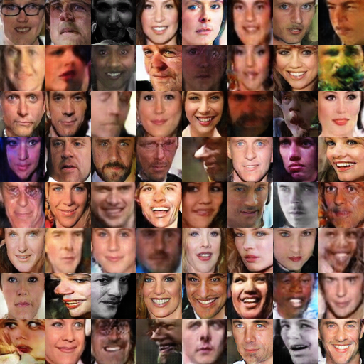
I’m training on the CASIA-WebFace and FaceScrub datasets because I had them on hand. After 14 epochs, the samples from mine look like:
Samples from my DCGAN after training for 14 epochs with the combined CASIA-WebFace and FaceScrub dataset.
You can also view the TensorFlow graphs and loss functions with TensorBoard.tensorboard --logdir ./logs
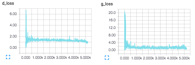
TensorBoard loss visualizations. Will be updated in real-time when training.
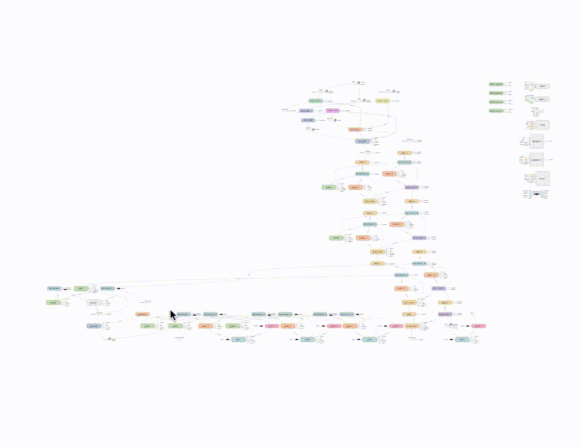
TensorBoard visualization of DCGAN networks.
Step 3: Finding the best fake image for image completionNow that we have a trained discriminator D(x)D(x) and
Image completion with DCGANs
generator G(z)G(z),
how can we use them to complete images? In this section I present the techniques in Raymond Yeh and Chen Chen et al.’s paper “Semantic Image
Inpainting with Perceptual and Contextual Losses,” which was just posted on arXiv on July 26, 2016.
To do completion for some image yy,
something reasonable that doesn’t work is to maximize D(y)D(y) over
the missing pixels. This will result in something that’s neither from the data distribution (pdatapdata)
nor the generative distribution (pgpg).
What we want is a reasonable projection of yy onto
the generative distribution.
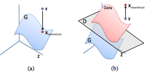
(a): Ideal reconstruction of yy onto
the generative distribution (the blue manifold). (b): Failure example of trying to reconstruct yy by
only maximizing D(y)D(y).
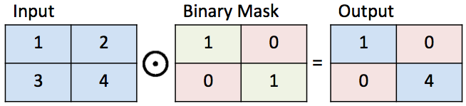
This image is from the inpainting paper.To define a reasonable projection, let’s first define some notation for completing images. We use a binary mask MM that
[ML-Heavy] Loss function for projecting onto pgpg
has values 0 or 1. A value of 1 represents the parts of the image we want to keep and a value of 0 represents the parts of the image we want to complete. We can now define how to complete an image yy given
the binary mask MM.
Multiply the elements of yy by
the elements of MM.
The element-wise product between two matrices is sometimes called the Hadamard product and is represented as M⊙yM⊙y. M⊙yM⊙ygives
the original part of the image.
Illustration of a binary mask.
Next, suppose we’ve found an image from the generator G(z^)G(z^) for
some z^z^ that
gives a reasonable reconstruction of the missing portions. The completed pixels (1−M)⊙G(z^)(1−M)⊙G(z^) can
be added to the original pixels to create the reconstructed image:
xreconstructed=M⊙y+(1−M)⊙G(z^)xreconstructed=M⊙y+(1−M)⊙G(z^)
Now all we need to do is find some G(z^)G(z^) that
does a good job at completing the image. To find z^z^,
let’s revisit our goals of recovering contextual and perceptual information from the beginning of this post and pose them in the context of DCGANs. We’ll do this by defining loss
functions for an arbitrary z∼pzz∼pz.
A smaller value of these loss functions means that zz is
more suitable for completion than a larger value.
Contextual Loss: To keep the same context as the input image, make sure the known pixel locations in the input image yy are
similar to the pixels in G(z)G(z).
We need to penalize G(z)G(z) for
not creating a similar image for the pixels that we know about. Formally, we do this by element-wise subtracting the pixels in yy from G(z)G(z) and
looking at how much they differ:
Lcontextual(z)=||M⊙G(z)−M⊙y||1,Lcontextual(z)=||M⊙G(z)−M⊙y||1,
where ||x||1=∑i|xi|||x||1=∑i|xi| is
the ℓ1ℓ1 norm of
some vector xx.
The ℓ2ℓ2 norm is
another reasonable choice, but the inpainting paper says that the ℓ1ℓ1 norm
works better in practice.
In the ideal case, all of the pixels at known locations are the same between yy and G(z)G(z).
Then G(z)i−yi=0G(z)i−yi=0 for
the known pixels iiand
thus Lcontextual(z)=0Lcontextual(z)=0.
Perceptual Loss: To recover an image that looks real, let’s make sure the discriminator is properly convinced that the image looks real. We’ll do this with the same criterion used in training the DCGAN:
Lperceptual(z)=log(1−D(G(z)))Lperceptual(z)=log(1−D(G(z)))
We’re finally ready to find z^z^ with
a combination of the contextual and perceptual losses:
L(z)≡Lcontextual(z)+λLperceptual(z)L(z)≡Lcontextual(z)+λLperceptual(z)
z^≡argminzL(z)z^≡argminzL(z)
where λλ is
a hyper-parameter that controls how import the contextual loss is relative to the perceptual loss. (I use λ=0.1λ=0.1 by
default and haven’t played with it too much.) Then as before, the reconstructed image fills in the missing values of yy with G(z^)G(z^):
xreconstructed=M⊙y+(1−M)⊙G(z^)xreconstructed=M⊙y+(1−M)⊙G(z^)
The inpainting paper also uses poisson blending (see
Chris Traile’s post for an introduction to it) to smooth the reconstructed image.This section presents the changes I’ve added to bamos/dcgan-completion.tensorflow that modifies Taehoon Kim’scarpedm20/DCGAN-tensorflow for
[ML-Heavy] TensorFlow implementation of image completion with DCGANs
image completion.
We can re-use a lot of the existing variables for completion. The only new variable we’ll add is a mask for completion:self.mask = tf.placeholder(tf.float32, [None] + self.image_shape, name='mask')
We’ll solve argminzL(z)argminzL(z) iteratively
with gradient descent with the gradients ∇zL(z)∇zL(z).
TensorFlow’s automatic differentiation can compute this for us once we’ve defined the loss functions! So the entire
idea of completion with DCGANs can be implemented by just adding four lines of TensorFlow code to an existing DCGAN implementation. (Of course implementing this also involves some non-TensorFlow code.)self.contextual_loss = tf.reduce_sum( tf.contrib.layers.flatten( tf.abs(tf.mul(self.mask, self.G) - tf.mul(self.mask, self.images))), 1) self.perceptual_loss = self.g_loss self.complete_loss = self.contextual_loss + self.lam*self.perceptual_loss self.grad_complete_loss = tf.gradients(self.complete_loss, self.z)
Next, let’s define a mask. I’ve only added one for the center portions of images, but feel free to add something else like a random mask and send in a pull request.if config.maskType == 'center': scale = 0.25 assert(scale <= 0.5) mask = np.ones(self.image_shape) l = int(self.image_size*scale) u = int(self.image_size*(1.0-scale)) mask[l:u, l:u, :] = 0.0
For gradient descent, we’ll use projected gradient descent with minibatches and momentum to project zz to
be in [−1,1][−1,1].for idx in xrange(0, batch_idxs): batch_images = ... batch_mask = np.resize(mask, [self.batch_size] + self.image_shape) zhats = np.random.uniform(-1, 1, size=(self.batch_size, self.z_dim)) v = 0 for i in xrange(config.nIter): fd = { self.z: zhats, self.mask: batch_mask, self.images: batch_images, } run = [self.complete_loss, self.grad_complete_loss, self.G] loss, g, G_imgs = self.sess.run(run, feed_dict=fd) v_prev = np.copy(v) v = config.momentum*v - config.lr*g[0] zhats += -config.momentum * v_prev + (1+config.momentum)*v zhats = np.clip(zhats, -1, 1)Select some images to complete and place them in
Completing your imagesdcgan-completion.tensorflow/your-test-data/raw.
Align them as before asdcgan-completion.tensorflow/your-test-data/aligned.
I randomly selected images from the LFW for this. My DCGAN wasn’t trained on any of the identities in the LFW.
You can run the completion on your images with:./complete.py ./data/your-test-data/aligned/* --outDir outputImages
This will run and periodically output the completed images to--outDir.
You can create create a gif from these with ImageMagick:cd outputImages convert -delay 10 -loop 0 completed/*.png completion.gif
Final image completions. The centers of these images are being automatically generated. The source code to create this is available here. These
are not curated! I selected a random subset of images from the LFW dataset.Thanks for reading, we made it! In this blog post, we covered one method of completing images that:
Conclusion
Interprets images as being samples from
a probability distribution.
Generates fake images.
Finds the best fake image for completion.
My examples were on faces, but DCGANs can be trained on other types of images too. In general, GANs are difficult to train and we don’t yet know how to train them on certain classes of objects, nor
on large images. However they’re a promising model and I’m excited to see where GAN research takes us!
Feel free to ping me on Twitter @brandondamos, Github @bamos,
or elsewhere if you have any comments or suggestions on this post. Thanks!
DCGAN samples (left) and improved GAN samples (right, not covered in this post) on ImageNet showing that we don’t yet understand how to use GANs on every type of image. This image is from the improved
GAN paper.Please consider citing this project in your publications if it helps your research. The following is a BibTeX and plaintext reference. The BibTeX
Citation for this article/project
entry requires theurlLaTeX package.@misc{amos2016image, title = {{Image Completion with Deep Learning in TensorFlow}}, author = {Amos, Brandon}, howpublished = {\url{http://bamos.github.io/2016/08/09/deep-completion}}, note = {Accessed: [Insert date here]} } Brandon Amos. Image Completion with Deep Learning in TensorFlow. http://bamos.github.io/2016/08/09/deep-completion. Accessed: [Insert date here]Raymond Yeh and Chen Chen et al. “Semantic Image Inpainting with Perceptual and Contextual Losses:” Paper this post was based
Partial bibliography for further reading
on.
D. Pathak et al. Context Encoders: Feature Learning by Inpainting at CVPR 2016: Another recent method
for inpainting that use similar loss functions and have released code on GitHub at pathak22/context-encoder. This method is
less computationally expensive than Yeh and Chen et al. because they use a single forward network pass instead of solving an optimization problem that involves many forward and backward passes.
Ian Goodfellow et al. “Generative Adversarial Nets”
Vincent Dumoulin and Francesco Visin. “A guide to convolution arithmetic for deep learning”
Alec Radford, Luke Metz, and Soumith Chintala. “Unsupervised Representation Learning with Deep Convolutional Generative Adversarial
Networks”
Emily Denton et al. “Deep Generative Image Models using a Laplacian Pyramid of Adversarial Networks:” Paper behind the
EyeScream Project.
Tim Salimans et al. “Improved Techniques for Training GANs:” OpenAI’s first paper. (Not discussed here.)As a machine learning researcher, I mostly use numpy, Torch, and TensorFlow in my programs. A few years ago,
Bonus: Incomplete Thoughts on TensorFlow and Torch
I used Fortran. I implemented OpenFace as a Python library in numpy that calls into networks trained with Torch. Over the past
few months, I’ve been using TensorFlow more seriously and have a few thoughts comparing Torch and TensorFlow. These are non-exhaustive and from my personal experiences as a user.
If I am misunderstanding something here, please message me and I’ll add a correction. Due to the fast-paced nature of these frameworks, it’s easy to not have references to everything.
There are many great collections of tutorials, pre-trained models, and technologies for both Torch and TensorFlow in projects like awesome-torch and awesome-tensorflow.
I haven’t used torchnet, but it seems promising.
Torch’s REPL is very nice and I always have it open when I’m developing in Torch to quickly try out operations. TensorFlow’sInteractiveSessionis
nice, but I find that trying things out interactively is a little slower since everything has to be defined symbolically and initialized in the session. I much prefer trying quick numpy operations in Python’s REPL over TensorFlow operations.
As with a lot of other programming, error messages in TensorFlow and Torch have their own learning curves. Debugging TensorFlow usually involves reasoning about the symbolic constructions while debugging Torch is more concrete. Sometimes
the error messages are confusing for me and I send in an issue only to find out that my error was obvious.
Having Python support is critical for my research. I love the scientific Python programming stack and libraries like matplotliband cvxpy that
don’t have an equivalent in Lua. This is why I wrote OpenFace to use Torch for training the neural network, but Python for everything
else.
I can easily convert TensorFlow arrays to numpy format and use them with other Python code, but I have to work hard to do this with Torch. When I tried using npy4th,
I found a bug (that I haven’t reported, sorry) that caused incorrect data to be saved.Torch’s hdf5 bindings seem to work well and
can easily be loaded in Python. And for smaller things, I just manually write out logs to a CSV file.
Torch has some equivalents to Python, like gnuplot wrappers for some plotting, but I prefer
the Python alternatives. There are some Python Torch wrappers like pytorch or lutorpy that
might make this easier, but I haven’t tried them and my impression is that they’re not able to cover every Torch feature that can be done in Lua.
In Torch, it’s easy to do very detailed operations on tensors that can execute on the CPU or GPU. With TensorFlow, GPU operations need to be implemented symbolically. In Torch, it’s easy to drop into native C or
CUDA if I need to add calls to a C or CUDA library. For example, I’ve created (CPU-only) Torch wrappers around the gurobi and ecos C
optimization libraries.
In TensorFlow, dropping into C or CUDA is definitely possible (and easy) on the CPU through numpy conversions, but I’m not sure how I would make a native CUDA call. It’s probably possible, but there are no documentation
or examples on this.
TensorFlow (built-in) and Torch’s nngraph package graph constructions are both nice. In my experiences for complex graphs,
TensorFlow is able to optimize the computations and executes about twice as fast as Torch. I love nngraph’s visualizations, they’re much clearer than TensorBoard’s in my experiences.
TensorBoard is convenient and okay, but I am currently not using
it for a few reasons. (In this post, I only used it becausecarpedm20/DCGAN-tensorflow uses it.) The plots are not publication-quality
and modifications are very limited. For example, it’s (currently) impossible to add a rolling average. The TensorBoard data is stored in a protobuf format and there’s
currently no documentation or examples on loading the data in my own script. My current solution is to just write out data to CSV files and load and plot them with another script.
I am not surprised to find bugs or missing features in Torch/Lua code. Here’s my PR removing an incorrect rank check
to the LAPACK potrs call. I also had to add a potrs wrapper for CUDA. Sometimes
I find minor bugs when using TensorFlow/tflearn, but not as frequently and they’re usually minor.
Automatic differentiation in TensorFlow is nice. I can define my loss with one line of code and then get the gradients with one more line. I haven’t used Torch’s
autograd package.
The Torch and TensorFlow communities are great at keeping up with the latest deep learning techniques. If a popular idea is released, Torch and TensorFlow implementations are quickly released.
Batch normalization is easier to use in Torch and in general it’s nice to not worry about explicitly defining all of my trainable variables like in TensorFlow. tflearn makes
this a little easier in TensorFlow, but I still prefer Torch’s way.
I am not surprised to learn about useful under-documented features in Torch and TensorFlow by reading through somebody else’s source code on GitHub. I described in my last
blog post that I found a under-documented way to reduce Torch model sizes in OpenFace.
I prefer how models can be saved and loaded in Torch by passing the object to a function that serializes it and saves it to a single file on disk. In TensorFlow, saving and loading the graph is still functionally the same, but a little more involved. Loading
Torch models on ARM is possible, but tricky. I don’t have experience loading TensorFlow models on ARM.
When using multiple GPUs, settingcutorch.setDeviceprogrammatically
in Torch is slightly easier than exporting theCUDA_VISIBLE_DEVICESenvironment
variable in TensorFlow.
TensorFlow’s long startup time is a slight annoyance if I want to quickly debug my code on small examples. In Torch, the startup time is negligible.
In Python, I like overriding the process name for long-running experiments with setproctitle so that I can remember
what’s running when I look at the running processes on my GPUs or CPUs. However in Torch/Lua, nobody on the mailing
list was able to help me do this. I also asked on a Lua IRC channel and somebody tried to help me, but we weren’t able to figure it out.
Torch’s argcheck has a serious
limitation when functions have more than 9 optional arguments. In Python, I’d like to start using mypy for simple argument checking, but
I’m not sure how well it works in practice with scientific Python.
I wrote gurobi and ecos wrappers
because there weren’t any LP or QP solvers in Torch. To my knowledge there still aren’t any other options.

相关文章推荐
- Pro Deep Learning with TensorFlow: A Mathematical Approach to Advanced Artificial Intelligence in Python
- Deep Learning algorithms with TensorFlow
- Deep Learning for Chatbots, Part 2 – Implementing a Retrieval-Based Model in Tensorflow
- 基于深度学习的图像分类Image classification with deep learning常用模型
- Word2Vec (Part 1): NLP With Deep Learning with Tensorflow (Skip-gram)
- Word2Vec (Part 2): NLP With Deep Learning with Tensorflow (CBOW)
- Word2Vec (Part 2): NLP With Deep Learning with Tensorflow (CBOW)
- Deep Learning for Chatbots, Part 2 – Implementing a Retrieval-Based Model in Tensorflow
- Word2Vec (Part 1): NLP With Deep Learning with Tensorflow (Skip-gram)
- DeepLab:深度卷积网络,多孔卷积 和全连接条件随机场 的图像语义分割 Semantic Image Segmentation with Deep Convolutional Nets, Atro
- 《Hands-on Machine Learning with Scikit-Learn and TensorFlow》 读书笔记
- TensorFlow和深度学习入门教程(TensorFlow and deep learning without a PhD)
- Machine Learning with Scikit-Learn and Tensorflow 7.2 Bagging和Pasting
- TensorFlow Machine Learning with Financial Data on Google Cloud Platform
- 深度学习教程 TensorFlow and Deep Learning Tutorials
- Incentivizing exploration in reinforcement learning with deep predictive models
- 斯坦福课程“CS 20SI:TensorFlow for Deep Learning Research”中文讲义(2)
- Machine Learning with Scikit-Learn and Tensorflow 6 决策树(章节目录)
- Machine Learning with Scikit-Learn and Tensorflow 7.7 特征重要程度
- Machine Learning with Scikit-Learn and Tensorflow 7.10 Stacking