R语言,ID4.5算法,实现离散型与连续型数据决策树构建及打印
2017-06-18 20:03
375 查看
本人的第一篇文章,趁着我们的数据挖掘课设的时间,把实现的决策树代码,拿出来分享下。有很多漏洞和缺陷,还有很多骇客思想的成分,但是总之,能实现,看网上的代码,能用的其实也没几个。废话不多说,直接看代码
特别鸣谢博主skyonefly的代码
附上链接:R语言决策树代码
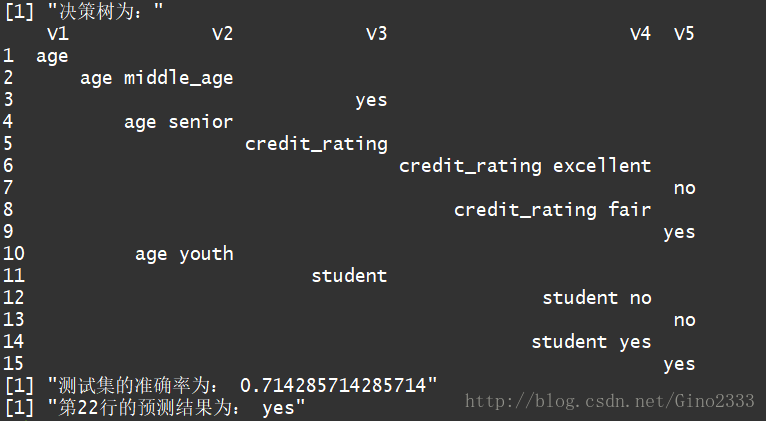
运行结果
下面是我用的数据
纯离散型
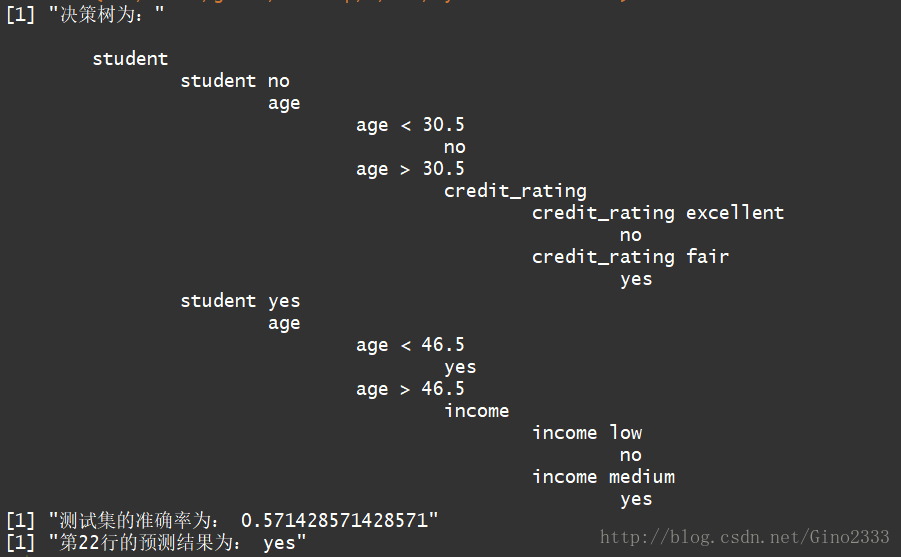
连续型+离散型
在文章的最后,我要感谢给予我动力和能量去完成这篇代码的人
特别鸣谢博主skyonefly的代码
附上链接:R语言决策树代码
#####
#####   ID4.5算法实现决策树
#####

#############################################Part1 基础函数#######################################################

#计算香农熵
calShannonEnt <- function(dataSet,labels){
numEntries<-length(dataSet[,labels])
key<-rep("a",numEntries)
for(i in 1:numEntries)
key[i]<-dataSet[i,labels]
shannonEnt<-0
prob<-table(key)/numEntries
for(i in 1:length(prob))
shannonEnt=shannonEnt-prob[i]*log(prob[i],2)
return(shannonEnt)
}

#划分数据集
splitDataSet <- function(dataSet,axis,value,tempSet = dataSet){
retDataSet = NULL
for(i in 1:nrow(dataSet)){
if(dataSet[i,axis] == value){
tempDataSet = tempSet[i,]
retDataSet = rbind(retDataSet,tempDataSet)
}
}
rownames(retDataSet) = NULL
return (retDataSet)
}

#选择信息增益最大的内部节点
chooseBestFeatureToSplita <- function(dataSet,labels, bestInfoGain){
numFeatures = ncol(dataSet) - 1
baseEntropy = calShannonEnt(dataSet,labels)
#最大信息增益
bestFeature = -1
for(i in  1: numFeatures){
featureLabels = levels(factor(dataSet[,i]))
# featureLabels = as.numeric(featureLabels)
newEntropy = 0.0
SplitInfo = 0.0
for( j in 1:length(featureLabels)){
subDataSet = splitDataSet(dataSet,i,featureLabels[j])
prob = length(subDataSet[,1])*1.0/nrow(dataSet)
newEntropy = newEntropy + prob*calShannonEnt(subDataSet,labels)
SplitInfo = -prob*log2(prob) + SplitInfo
}
infoGain = baseEntropy - newEntropy
GainRadio = infoGain/SplitInfo
if(SplitInfo > 0){
GainRadio = infoGain/SplitInfo
if(GainRadio > bestInfoGain){
bestInfoGain = infoGain
bestFeature = i
}
}
}
return (bestFeature)
}

#返回频数最高的列标签
majorityCnt <- function(classList){
classCount = NULL
count = as.numeric(table(classList))
majorityList = levels(as.factor(classList))
if(length(count) == 1){
return (majorityList[1])
}else{
f = max(count)
return (majorityList[which(count == f)][1])
}
}

#判断类标签是否只有一个因子水平
oneValue <- function(classList){
count = as.numeric(table(classList))
if(length(count) == 1){
return (TRUE)
}else
return (FALSE)
}

#树的打印
printTree <- function(tree){
df <- data.frame()
col <- 1
point <- c()
count <- 0
for(i in 1:length(tree)){
if(rownames(tree)[[i]] == 'labelFeature'){
df[i,col] = tree[[i]]
col = col + 1
count = count + 1
point[count] = col
names(point)[count] = tree[[i]]
}else if(rownames(tree)[[i]] == 'FeatureValue'){
for(j in 1:length(point)){
len = grep(names(point)[j],tree[[i]])
if(length(len) >= 1){
col = point[j]
}
}
df[i,col] = tree[[i]]
col = col + 1
}else{
df[i,col] = tree[[i]]
col = col + 1
}
}
for(i in 1:nrow(df)){
for(j in 1:ncol(df)){
if(is.na(df[i,j])){
df[i,j] = ""
}
}
}
return(df)
}

numericCol <- NULL

#加载数据
load <- function(filePath){
dataSet<-read.table(filePath,header = T)

dataSet = dataSet[,-1]

numericCol <<- c()
for(i in 1:length(ncol(dataSet))){
if(is.numeric(dataSet[,i])){
numericCol[i] <<- colnames(dataSet)[i]
}
}

dataSet = as.matrix(dataSet)

trainSet = dataSet[1:14,]
testSet = dataSet[15:21,]
preSet = dataSet[22,,drop=FALSE]
result = list(trainSet,testSet,preSet)
return (result)
}

#############################################Part2 连续值处理#####################################################

#将数据集全部转换成离散型
toDiscrete <- function(numericCol,dataSet,labels){

s <- c()
if(length(numericCol)>0){
for(i in 1:length(numericCol)){
if(numericCol[i] %in% colnames(dataSet)){
atr = dataSet[,numericCol[i]]
atr = as.numeric(atr)
Split = BestSplit(dataSet,numericCol[i],labels)#计算最佳分裂点
s[i] = Split
names(s)[i] = numericCol[i]
dataSet[,numericCol[i]] = toDiscreteCol(atr, Split)#将新离散型数据的写入dataSet
}
}
}

result = list(dataSet,s)
return(result)
}

#计算基尼系数
jini <- function(data,labels){
nument<-length(data[,1])
key<-rep("a",nument)
for(i in 1:nument) {
key[i]<-data[i,labels]
}

ent<-0
prob<-table(key)/nument
for(i in 1:length(prob))
ent=ent+prob[i]*prob[i]
ent = 1 - ent
return(ent)
}

#找到基尼系数最小的中值,作为分裂点
BestSplit <- function(dataSet,colname,labels){
numFeatures = nrow(dataSet) - 1
bestSplit = -1
sorted = sort(as.numeric(dataSet[,colname]))
atr = dataSet[,colname]
bestGini = 999
for(i in  1: numFeatures){
middle = (sorted[i] + sorted[i+1])/2
tempCol = toDiscreteCol(atr,middle)
dataSet[,colname] = tempCol
featureLabels = levels(factor(dataSet[,colname]))

Gini = 0.0
for( j in 1:length(featureLabels)){
subDataSet = splitDataSet(dataSet,colname,featureLabels[j])
prob = length(subDataSet[,1])*1.0/nrow(dataSet)
Gini = Gini + prob*jini(subDataSet,labels)
}

if(Gini <= bestGini){
bestGini = Gini
count = middle
}
}
return (count)
}

#将该列转换成离散型
toDiscreteCol <- function(atr, Split){
str <- c()
for(i in 1:length(atr)){
if(atr[i] <= Split){
str[i] = 'a'
}else{
str[i] = 'b'
}
}
return(str)
}

#############################################Part3 决策树的构建###################################################

#递归建立生成树
creatTree <- function(dataSet,labels,bestInfoGain){
result = toDiscrete(numericCol,dataSet,labels)
tempSet = dataSet
dataSet = result[[1]]
Split = result[[2]]
decision_tree = list()
classList = dataSet[,labels]

#判断是否属于同一类
if(oneValue(classList)){
label = classList[1]
return (rbind(decision_tree,label))
}

#是否在矩阵中只剩Label标签了,若只剩Label标签,则都分完了
if((ncol(dataSet) == 1)){
label = majorityCnt(classList)
decision_tree = rbind(decision_tree,labels)
return (decision_tree)
}

#选择bestFeature作为分割属性
bestFeature = chooseBestFeatureToSplita(dataSet,labels,bestInfoGain)
bestFeatureName = colnames(dataSet)[bestFeature]

#所有信息增益都小于bestInfoGain
if(bestFeature == -1){
label = majorityCnt(classList)
decision_tree = rbind(decision_tree,label)
return (decision_tree)
}
labelFeature = colnames(dataSet)[bestFeature]

#添加内部节点
decision_tree = rbind(decision_tree,labelFeature)

#选中了那个标签作为此次分类标签
attriCol = dataSet[,bestFeature]

temp_tree = data.frame()
stayData = dataSet
factor=levels(as.factor(attriCol))

for(j in 1:length(factor)){

#分裂成小数据集
dataSet = splitDataSet(stayData,bestFeature,factor[j],tempSet)

if(bestFeatureName %in% numericCol){
if(factor[j] == 'a'){
character = '<'
}else{
character = '>'
}
numpd = paste(character,Split[bestFeature])
FeatureValue = paste(bestFeatureName,numpd)
}else{
FeatureValue = paste(bestFeatureName,factor[j])
}

decision_tree = rbind(decision_tree, FeatureValue )

#删除已使用属性列
dataSet = dataSet[,-bestFeature,drop=FALSE]

#递归调用这个函数
temp_tree = creatTree(dataSet,labels,bestInfoGain)

decision_tree = rbind(decision_tree,temp_tree)
}
return (decision_tree)
}

#############################################Part4 预测函数#######################################################

#算正确率
test <- function(testSet,labels){
count <- 0
for(i in 1:nrow(testSet)){
pre = predict(testSet[i,,drop=FALSE],myTree)
if(is.null(pre)){
}else{
if(pre == testSet[i,labels]){
count = count + 1
}
}
}
return(count/nrow(testSet))
}

#打印预测结果
pre <- function(testSet){
for(i in 1:nrow(testSet)){
pre = predict(testSet[i,,drop=FALSE],myTree)
return(pre)
}
}

#预测函数
predict <- function(testSet, df, row = 1, col = 1){

if(df[row,col] == "yes"| df[row,col] == "no"){
return(df[row,col])
}else{
if(length(grep(" ",df[row,col])) == 0 & nchar(df[row,col]) > 0){
labelFeature = df[row,col]#获取属性名称
FeatureValue = testSet[,labelFeature][1]#获取属性值
if(labelFeature %in% numericCol){
count <- 1
rows <- c()
Split <- NULL
for(i in row:nrow(df)){
if(count > 2){
break
}
if(nchar(df[i,col+1]) > 0){
Split = as.numeric(strsplit(df[i,col+1]," ")[[1]][3])
rows[count] = i
count = count + 1
}
}

if(as.numeric(FeatureValue) < Split){
prediction = predict(testSet, df, rows[1] + 1, col + 2)
}else{
prediction = predict(testSet, df, rows[2] + 1, col + 2)
}
return(prediction)

}else{
sum = paste(labelFeature, FeatureValue)
for(i in row:nrow(df)){
if(df[i,col+1] == sum){
row = i
break
}
}
prediction = predict(testSet, df, row + 1, col + 2)
return(prediction)
}

}
}
}

###########################################Part5 加载数据并运行###################################################

#加载数据
myData = load("C:/Users/gino2/Desktop/R/DecisiontreeSampledata.txt")
#"D:/littlestar/DecisiontreeSampledata.txt"    离散型数据
#"D:/littlestar/DecisiontreeSampledataContinue.txt"    连续型数据

#创建决策树
#三个参数:训练数据集,类标签列,增益率的阈值
tree = creatTree(myData[[1]],'buys_computer',0.12)
myTree <- printTree(tree)
print(myTree)

#预测函数
rightProb = test(myData[[2]],'buys_computer')
print(paste("测试集的准确率为:",rightProb))

print(paste("第22行的预测结果为:",pre(myData[[3]])))
运行结果
下面是我用的数据
纯离散型
ID  age income  student credit_rating    buys_computer
1    youth   high   no   fair   no
2    youth   high   no   excellent  no
3    middle_age      high   no   fair   yes
4    senior      medium     no   fair   yes
5    senior     low yes  fair   yes
6    senior     low yes  excellent  no
7    middle_age     low yes  excellent  yes
8    youth   medium     no   fair   no
9    youth  low yes  fair   yes
10   senior      medium     yes  fair   yes
11   youth   medium     yes  excellent  yes
12   middle_age      medium     no   excellent  yes
13   middle_age      high   yes  fair   yes
14   senior      medium     no   excellent  no
15  youth    medium     no   fair   no
16  youth   low yes  excellent  yes
17   middle_age      medium     yes  fair   yes
18   middle_age      high   no   excellent  yes
19   middle_age     low no   excellent  yes
20   senior     low yes  excellent  yes
21   senior     high    no   fair   no
22   middle_age      medium     no   fair   NA
连续型+离散型
Id  age income  student credit_rating buys_computer
1   16  high    no  fair    no
2   25  high    no  excellent   no
3   34  high    no  fair    yes
4   41  medium  no  fair    yes
5   45  low yes fair    yes
6   48  low yes excellent   no
7   39  low yes excellent   yes
8   27  medium  no  fair    no
9   25  low yes fair    yes
10  49  medium  yes fair    yes
11  18  medium  yes excellent   yes
12  36  medium  no  excellent   yes
13  38  high    yes fair    yes
14  50  medium  no  excellent   no
15  19  medium  no  fair    no
16  25  low yes excellent   yes
17  35  medium  yes fair    yes
18  31  high    no  excellent   yes
19  38  low no  excellent   yes
20  45  low yes excellent   yes
21  43  high    no  fair    no
22  36  medium  no  fair    NA
在文章的最后,我要感谢给予我动力和能量去完成这篇代码的人

相关文章推荐
- 数据挖掘-决策树ID3分类算法的C++实现
- 机器学习入门算法及其java实现-ID3(决策树)算法
- 数据挖掘领域十大经典算法 --- 决策树算法 ID3/C4.5
- 数据挖掘—决策树ID3分类算法的C++实现
- 机器学习与数据挖掘算法 1.编程实现ID3算法,针对下表数据,生成决策树。
- 【年终分享】彩票数据预测算法(一):离散型马尔可夫链模型实现【附C#代码】
- pyhon实现决策树(ID3)算法进行数据的分类预测
- 数据挖掘-决策树ID3分类算法的C++实现
- 十大数据挖掘算法的R语言实现
- 数据挖掘-决策树ID3分类算法的C++实现
- 数据挖掘-决策树ID3分类算法的C++实现
- C++ 实现决策树 ID3 算法
- ID3 算法实现决策树
- 数据挖掘之决策树归纳算法的Python实现
- 数据挖掘-决策树ID3分类算法的C++实现
- 机器学习算法(二)——决策树分类算法及R语言实现方法
- [置顶] 数据挖掘常用算法理解与R语言实现(系列待完成)
- 数据分析之美:决策树R语言实现
- 数据挖掘-决策树ID3分类算法的C++实现
- 十大数据挖掘算法的R语言实现