【从传统方法到深度学习】图像分类
2017-06-17 16:57
519 查看
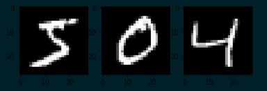
Kaggle上有一个图像分类比赛Digit Recognizer,数据集是大名鼎鼎的MNIST——图片是已分割 (image segmented)过的28*28的灰度图,手写数字部分对应的是0~255的灰度值,背景部分为0。
手写数字图片是长这样的:
手写数字识别可以看做是一个图像分类问题——对二维向量的灰度图进行分类。
思路比较简单:将二维向量拉直成一个一维向量,基于距离度量以判断向量间的相似性。显而易见,这种不带特征提取的朴素办法,丢掉了二维向量中最重要的四周相邻像素的信息。在比较干净的数据集MNIST还有不错的表现,准确率为96.927%。此外,kNN模型训练慢。
MLP
多层感知器MLP (Multi Layer Perceptron)亦即三层的前馈神经网络,所采用的特征与kNN方法类似——每一个像素点的灰度值对应于输入层的一个神经元,隐藏层的神经元数为700(一般介于输入层与输出层的数量之间),迭代次数epochs设为100。sklearn的MLPClassifier实现MLP分类,下面给出基于keras的MLP实现。没怎么细致地调参,准确率大概在98.530%左右。
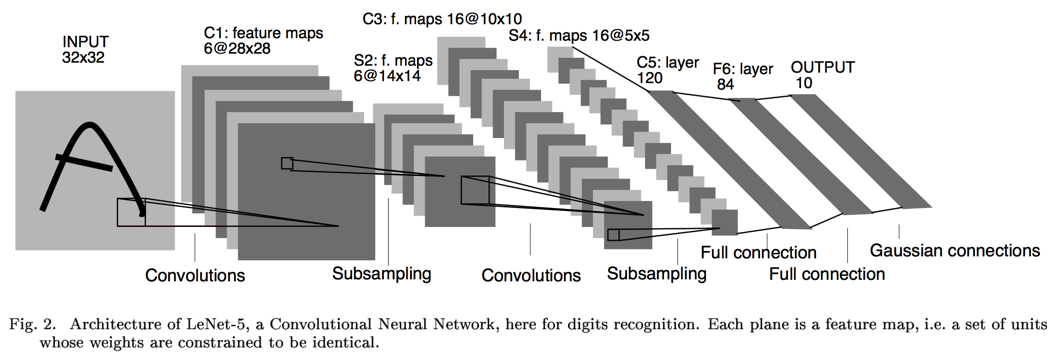
卷积、池化、卷积、池化,然后套2个全连接层,最后接个Guassian连接层。众所周知,CNN自带特征提取功能,不需要刻意地设计特征提取器。基于keras,Lenet-5 非正式实现如下:
对比以上三种方法的准确率,总结如下:
[2] LeCun, Yann, et al. "Gradient-based learning applied to document recognition." Proceedings of the IEEE 86.11 (1998): 2278-2324.
[3] Taylor B. Arnold,
Computer vision: LeNet-5, AlexNet, VGG-19, GoogLeNet.
from keras.datasets import mnist

(x_train, y_train), (x_test, y_test) = mnist.load_data()
x_train[0] # .shape = 28*28
"""
[[  0   0   0   0   0   0   0   0   0   0   0   0   0   0   0   0   0   0
0   0   0   0   0   0   0   0   0   0]
...
[  0   0   0   0   0   0   0   0   0   0   0   0   3  18  18  18 126 136
175  26 166 255 247 127   0   0   0   0]
[  0   0   0   0   0   0   0   0  30  36  94 154 170 253 253 253 253 253
225 172 253 242 195  64   0   0   0   0]
...
[  0   0   0   0   0   0   0   0   0   0   0   0   0   0   0   0   0   0
0   0   0   0   0   0   0   0   0   0]]
"""
手写数字图片是长这样的:
import matplotlib.pyplot as plt

plt.subplot(1, 3, 1)
plt.imshow(x_train[0], cmap='gray')
plt.subplot(1, 3, 2)
plt.imshow(x_train[1], cmap='gray')
plt.subplot(1, 3, 3)
plt.imshow(x_train[2], cmap='gray')
plt.show()
手写数字识别可以看做是一个图像分类问题——对二维向量的灰度图进行分类。
2. 识别
Rodrigo Benenson给出50种方法在MNIST的错误率。本文将从传统方法过渡到深度学习,对比准确率来看。以下代码基于Python 3.6 + sklearn 0.18.1 + keras 2.0.4。传统方法
kNN思路比较简单:将二维向量拉直成一个一维向量,基于距离度量以判断向量间的相似性。显而易见,这种不带特征提取的朴素办法,丢掉了二维向量中最重要的四周相邻像素的信息。在比较干净的数据集MNIST还有不错的表现,准确率为96.927%。此外,kNN模型训练慢。
from sklearn import neighbors
from sklearn.metrics import precision_score

num_pixels = x_train[0].shape[0] * x_train[0].shape[1]
x_train = x_train.reshape((x_train.shape[0], num_pixels))
x_test = x_test.reshape((x_test.shape[0], num_pixels))

knn = neighbors.KNeighborsClassifier()
knn.fit(x_train, y_train)
pred = knn.predict(x_test)
precision_score(y_test, pred, average='macro') # 0.96927533865705706
MLP
多层感知器MLP (Multi Layer Perceptron)亦即三层的前馈神经网络,所采用的特征与kNN方法类似——每一个像素点的灰度值对应于输入层的一个神经元,隐藏层的神经元数为700(一般介于输入层与输出层的数量之间),迭代次数epochs设为100。sklearn的MLPClassifier实现MLP分类,下面给出基于keras的MLP实现。没怎么细致地调参,准确率大概在98.530%左右。
from keras.layers import Dense
from keras.models import Sequential
from keras.utils import np_utils

# normalization
num_pixels = 28 * 28
x_train = x_train.reshape(x_train.shape[0], num_pixels).astype('float32') / 255
x_test = x_test.reshape(x_test.shape[0], num_pixels).astype('float32') / 255
# one-hot enconder for class
y_train = np_utils.to_categorical(y_train)
y_test = np_utils.to_categorical(y_test)
num_classes = y_train.shape[1]

model = Sequential([
Dense(700, input_dim=num_pixels, activation='relu', kernel_initializer='normal'),  # hidden layer
Dense(num_classes, activation='softmax', kernel_initializer='normal')  # output layer
])
model.compile(optimizer='adam', loss='categorical_crossentropy', metrics=['accuracy'])
model.summary()

model.fit(x_train, y_train, validation_data=(x_test, y_test), epochs=600, batch_size=200, verbose=2)
model.evaluate(x_test, y_test, verbose=0)  # [0.10381294689745164, 0.98529999999999995]
深度学习
LeCun早在1989年发表的论文 [1]中提出了用CNN (Convolutional Neural Networks)来做手写数字识别,后来 [2]又改进到Lenet-5,其网络结构如下图所示:卷积、池化、卷积、池化,然后套2个全连接层,最后接个Guassian连接层。众所周知,CNN自带特征提取功能,不需要刻意地设计特征提取器。基于keras,Lenet-5 非正式实现如下:
import keras
from keras.layers import Conv2D, MaxPooling2D
from keras.layers import Dense, Dropout, Flatten, Activation
from keras.models import Sequential
from keras.utils import np_utils

img_rows, img_cols = 28, 28
# TensorFlow backend: image_data_format() == 'channels_last'
x_train = x_train.reshape(x_train.shape[0], img_rows, img_cols, 1).astype('float32') / 255
x_test = x_test.reshape(x_test.shape[0], img_rows, img_cols, 1).astype('float32') / 255
# one-hot code for class
y_train = np_utils.to_categorical(y_train)
y_test = np_utils.to_categorical(y_test)
num_classes = y_train.shape[1]

model = Sequential()
model.add(Conv2D(filters=6, kernel_size=(5, 5), padding='valid', input_shape=(28, 28, 1)))
model.add(MaxPooling2D(pool_size=(2, 2)))
model.add(Activation("sigmoid"))

model.add(Conv2D(16, kernel_size=(5, 5), padding='valid'))
model.add(MaxPooling2D(pool_size=(2, 2)))
model.add(Activation("sigmoid"))
model.add(Dropout(0.25))
# full connection
model.add(Conv2D(120, kernel_size=(1, 1), padding='valid'))
model.add(Flatten())
# full connection
model.add(Dense(84, activation='sigmoid'))
model.add(Dense(num_classes, activation='softmax'))

model.compile(loss=keras.losses.categorical_crossentropy,
optimizer=keras.optimizers.SGD(lr=0.08, momentum=0.9),
metrics=['accuracy'])
model.summary()
model.fit(x_train, y_train, batch_size=32, epochs=8,
verbose=1, validation_data=(x_test, y_test))
model.evaluate(x_test, y_test, verbose=0)
对比以上三种方法的准确率,总结如下:
| 特征 | 分类器 | 准确率 |
|---|---|---|
| gray | kNN | 96.927% |
| gray | 3-layer neural networks | 98.530% |
| Lenet-5 | 98.640% |
3. 参考资料
[1] LeCun, Yann, et al. "Backpropagation applied to handwritten zip code recognition." Neural computation 1.4 (1989): 541-551.[2] LeCun, Yann, et al. "Gradient-based learning applied to document recognition." Proceedings of the IEEE 86.11 (1998): 2278-2324.
[3] Taylor B. Arnold,
Computer vision: LeNet-5, AlexNet, VGG-19, GoogLeNet.

相关文章推荐
- 专访 | 清华大学朱军:深度学习“盛行”_传统方法何去何从?
- 深度学习笔记——基于传统机器学习算法(LR、SVM、GBDT、RandomForest)的句子对匹配方法
- 专访 | 清华大学朱军:深度学习“盛行”_传统方法何去何从?
- 【从传统方法到深度学习】图像分类
- 【从传统方法到深度学习】情感分析
- 新闻上的文本分类:机器学习大乱斗 王岳王院长 王岳王院长 5 个月前 目标 从头开始实践中文短文本分类,记录一下实验流程与遇到的坑 运用多种机器学习(深度学习 + 传统机器学习)方法比较短文本分类处
- 深度学习优化方法:梯度下降法及其变形
- 【深度学习】数据降维方法总结
- struts学习:传统方法完成struts注册表单校验与回显数据
- 深度学习、自然语言处理和表征方法
- 深度学习中的数据预处理方法
- 深度学习卷积算法的GPU加速实现方法
- 深度学习防止过拟合的方法
- 深度学习--防止过拟合的几种方法
- 深度学习——Xavier初始化方法
- 从SRCNN到EDSR,总结深度学习端到端超分辨率方法发展历程
- 深度学习笔记(五) 代价函数的梯度求解过程和方法
- R-CNN,SPP-NET, Fast-R-CNN,Faster-R-CNN, YOLO, SSD系列深度学习检测方法梳理
- TensorFlow Saver方法 深度学习 输出模型
- 深度学习(Deep Learning)的基本思想和方法,入门介绍