An Introduction to CNN based Object Detection

1. Content

Brief Revisit to the “Ancient” Algorithm

HOG (before *2007)

DPM (*2010~2014)

Epochal Evolution of R-CNN

R-CNN *2014

Fast-RCNN *2015

Faster-RCNN *2015

Efficient One-shot Methods

YOLO

SSD

Others

2. Brief Revisit to the “Ancient” Algorithm

2.1 Histograms of Gradients (HOG)

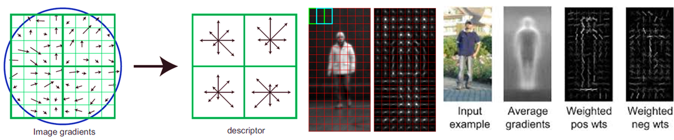
Calculate gradient for each pixel

For each Cell, a histogram of gradient is computed

For each Block, a HOG feature is extracted by concatenating histograms of each Cell

If Block size = 16*16, Block stride = 8, Cell size = 8*8, Bin size = 9, Slide-window size = 128*64, then HOG feature is a 3780-d feature. #Block=((64-16)/8+1)*((128-16)/8+1)=105, #Cell=(16/8)*(16/8)=4, 105*4*9=3780

2.2 Deformable Part Models (DPM)

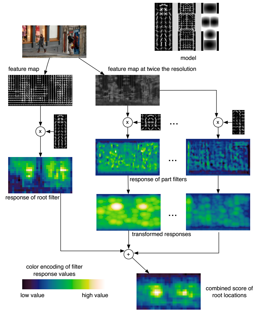
Di,l(x,y)=maxdx,dy(Ri,l(x+dx,y+dy)−di⋅ϕd(dx,dy))

This transformation spreads high filter scores to nearby locations, taking into account the deformation costs.

score(x0,y0,l0)=R−0,l0(x0,y0)+∑i=1nDi,l0−λ(2(x0,y0)+vi)+b

The overall root scores at each level can be expressed by the sum of the root filter response at that level, plus shifted versions of transformed and sub-sampled part responses.

3. Epochal Evolution of R-CNN

3.1 RCNN

3.1.1 Regions with CNN Features

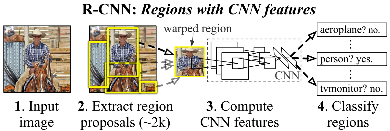
Region proposals (Selective Search, ~2k)

CNN features (AlexNet, VGG-16, warped region in image)

Classifier (Linear SVM per class)

Bounding box (Class-specific regressor)

Run-time speed (VGG-16, 47 s/img on single K40 GPU)

3.1.2 Experiment Result (AlexNet)

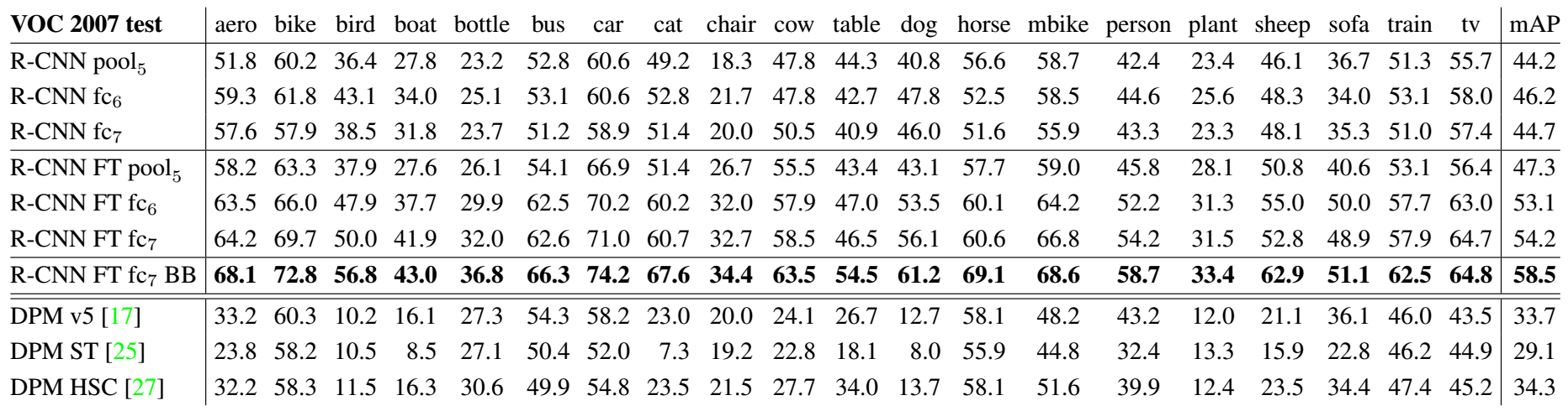
Without FT, fc7 is worse than fc6, pool5 is quite competitive. Much of the CNN’s representational power comes from its convolutional layers, rather than from the much larger densely connected layers.

With FT, The boost from fine-tuning is much larger for fc6 and fc7 than for pool5. Pool5 features are general. Learning domain-specific non-linear classifiers helps a lot.

Bounding box regression helps reduce localization errors.

3.1.3 Interesting Details – Training

Pre-trained on ILSVRC2012 classification task

Fine-tuned on proposals with N+1 classes without any modification to the network

IOU>0.5 over ground-truth as positive samples, others as negative samples

Each mini-batch contains 32 positive samples and 96 background samples

SVM for each category

Ground-truth window as positive samples

IOU<0.3 over ground-truth as negative samples

Hard negative mining is adopted

Bounding-box regression

Class-specific

Features computed by CNN

Only the proposals IOU>0.6 overlap ground-truth

Coordinates in pixel

3.1.4 Interesting Details – FP Error Types

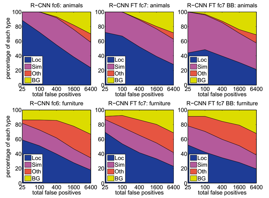
Loc: poor localization, 0.1 < IOU < 0.5

Sim: confusion with a similar category

Oth: confusion with a dissimilar object category

BG: a FP that fired on background

3.2 Fast-RCNN

3.2.1 What’s Wrong with RCNN

Training is a multi-stage pipeline (Proposal, Fine-tune, SVMs, Regressors)

Training is expensive in space and time (Extract feature from every proposal, Need to save to disk)

Oject detection is slow (47 s/img on K40)

3.2.2 R-CNN with ROI Pooling

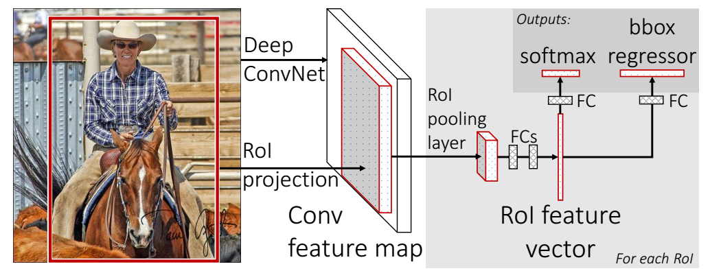
Region proposals (Selective Search, ~2k)

CNN features (AlexNet, VGG-16, ROI in feature map)

Classifier (sub-network softmax)

Bounding box (sub-network regressor)

Run-time speed (VGG-16, 0.32 s/img on single K40 GPU)

3.2.3 ROI Pooling

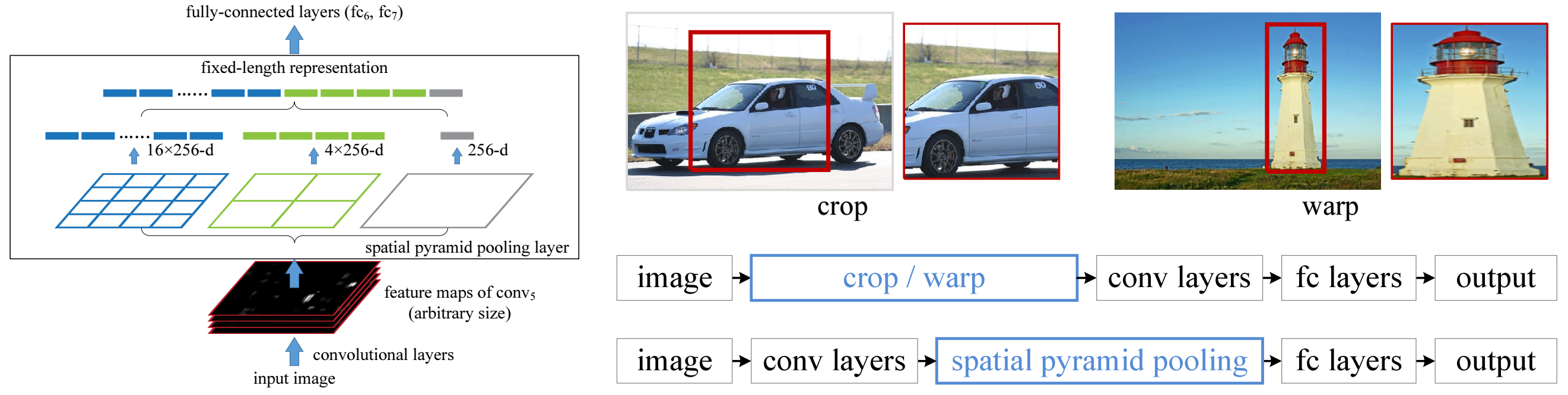
Inspired by Spatial Pyramid Pooling (SPPNet)

Convert arbitrary input size to fixed length

The input is an ROI area in feature map

The input is divided into grids

In each grid, pooling is used to extract features

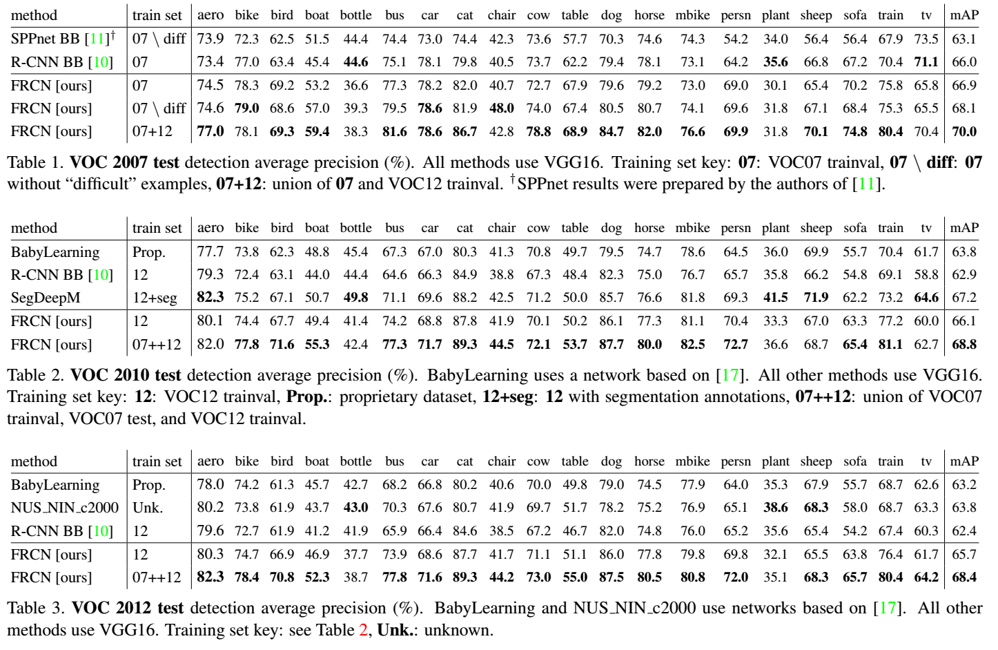
3.2.4 Experiment Result (VGG16)

3.2.5 Interesting Details – Training

Pre-trained on ILSVRC2012 classification task

Fine-tuned with N+1 classes and two sibling layers



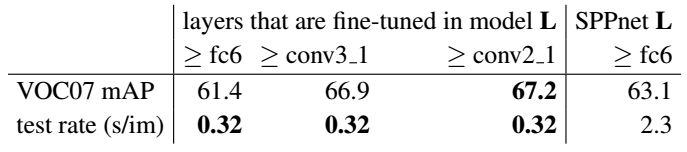
Fine-tune the whole network

Each mini-batch has 2 images and 64 ROIs from each images

25% of the ROIs have IOU>0.5 with ground-truth as positive samples

The rest of the ROIs have IOU [0.1, 0.5) with ground-truth as background samples

L(p,u,lu,v)=Lcls(p,u)+λ[u≥1]Lloc(tu,v)

Multi-task loss, one loss for classification and one for bounding box regression

ROI pooling back-propagation is similar with max-pooling

Accelerate using truncated SVD



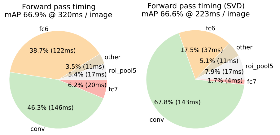
Implemented by using two FCs without non-linear activation

Training time

146x faster than R-CNN

If accelerated with truncated SVD, 213x faster than R-CNN

3.2.6 Interesting Details – Design evaluation

Does multi-task training help? Yes, it does!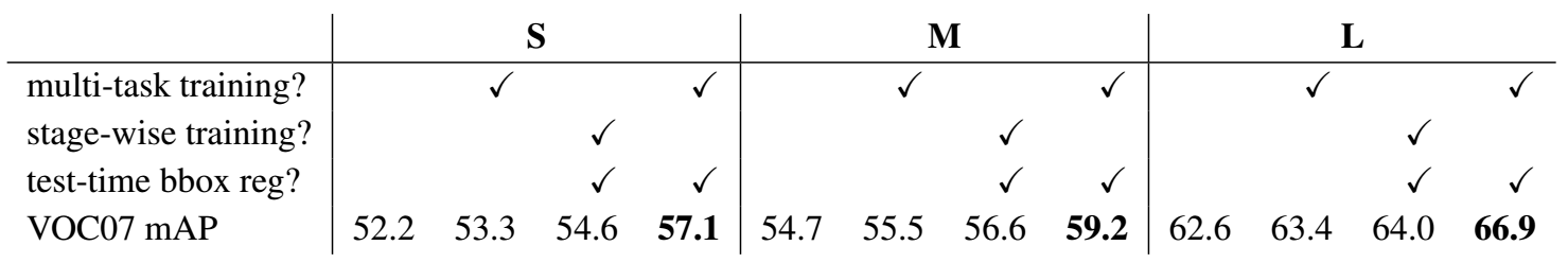



Test with multiple scales? Yes but with cost.



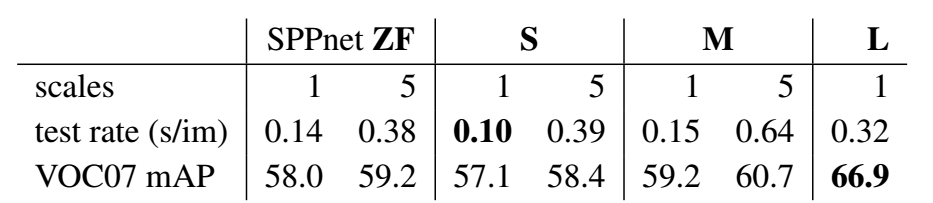
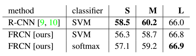
Do SVMs outperform softmax? Interesting…

3.3 Faster-RCNN

3.3.1 Room to improve Fast-RCNN

Region proposal has become the bottleneck

2s for Selective Search, 0.320s for Fast-RCNN

Why not a unified end-to-end framework

3.3.2 Fast-RCNN with RPN (Region Proposal Network)

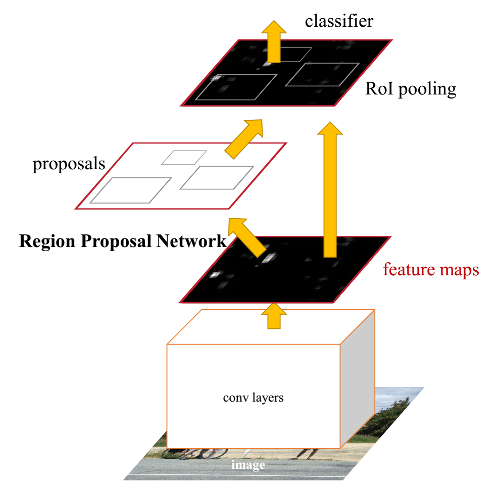
Region proposals (RPN, ~300)

Classifier (sub-network softmax)

Bounding box (RPN regressor, sub-network regressor)

Run-time speed (VGG-16, 0.198 s/img on single K40 GPU)

3.3.3 Region Proposal Network

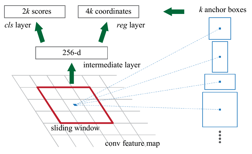
Anchors

reference box, prior box, default box

Works in a slide-window way

Implemented by 3*3 kernel convolution

Centered at the slide-window

Translation-Invariant

If objects translated, proposal should be translated

Translated along slide-window

Multi-Scale and Multi-Ratio

A pyramid of anchors

A set of different ratios

Relies on single scale feature map

Objectness and Localization

Two siblings

Objectness score

Bounding box regression

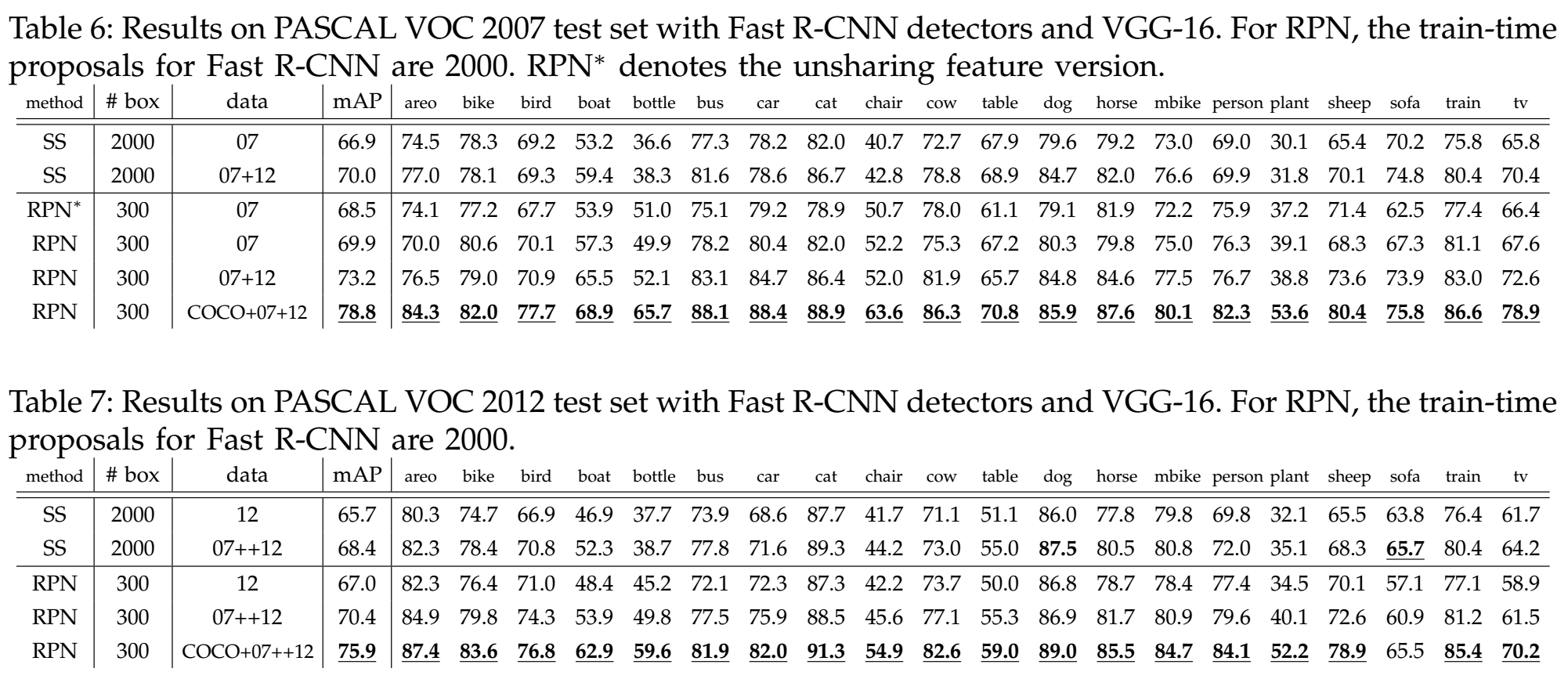
3.3.4 Experiment Result

3.3.5 Interesting Details – Training

Sharing Features for RPN and Fast-RCNN

Alternating training

Approximate joint training

Non-approximate joint training

Alternating Training

Train RPN(@) using pre-trained model

Train Fast-RCNN(#) using pre-trained model and @’s proposal

Train RPN($) using #’s weight with shared layers fixed

Train Fast-RCNN using $’s proposal with shared layers fixed

Training RPN

Each mini-batch arises from a single image

Positive samples: the anchors with (1) the highest IOU and (2) IOU>0.7 overlap with any ground-truth

Negative samples: IOU<0.3 overlap with all ground-truth

Randomly sample 256 anchors, pos:neg = 1:1

Loss function with Ncls=256, Nreg=~2400, λ=10

Anchors cross image boundaries do not contribute at training stage

3.3.6 Interesting Details – Design Evaluation

Ablation on RPN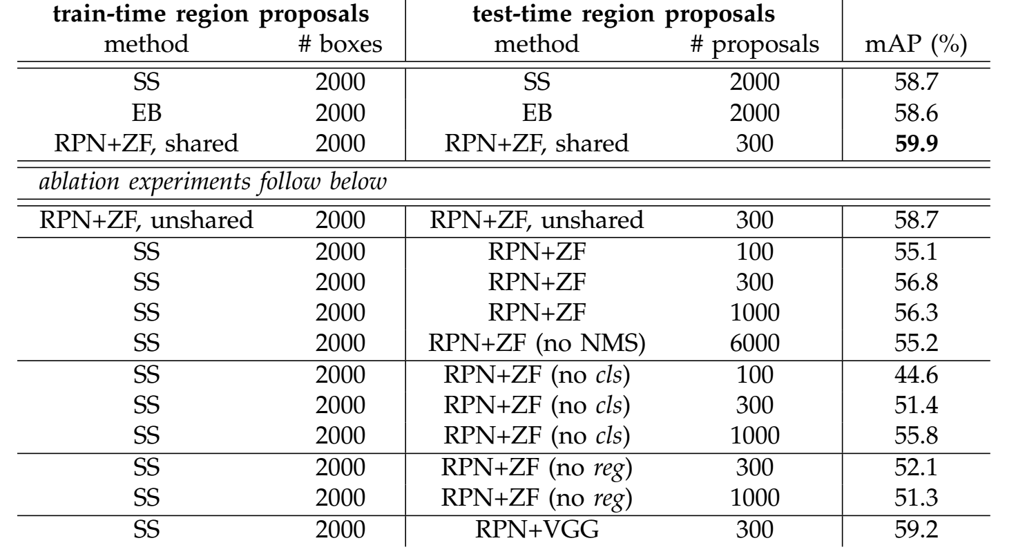



Sharing: Detector feature helps RPN

RPN generate quite good proposals

No cls, randomly selecting proposal, score matters

No reg, worse localization error

Timing



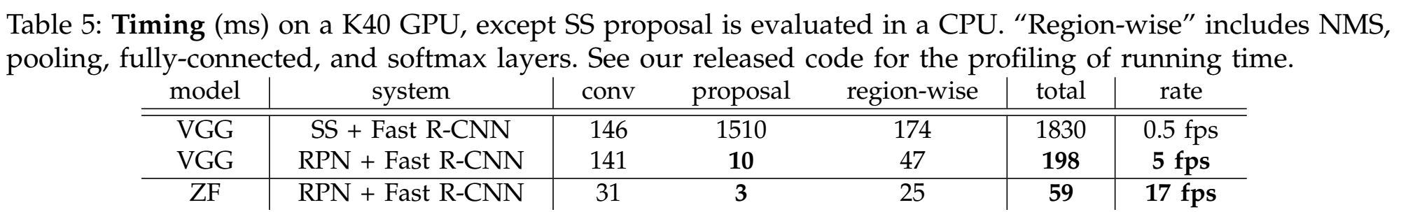
Nearly cost free

Less proposal

Anchors



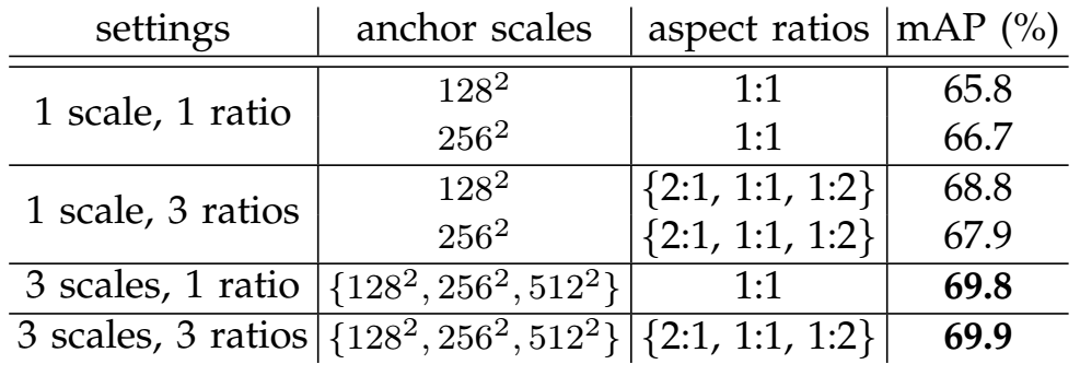
Scale is more effective

4 Efficient One-shot Methods

4.1 YOLO

4.1.1 You Only Look Once

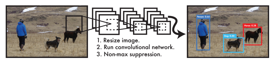
A simple forward on the full image (almost same with a classification task)

Frame object detection as a regression problem (bounding box coordinates, class probabilities)

Extremely fast (45 fps for base network, or 150 fps for fast version)

Reasoning globally on the full context (no slide-window or region proposals)

Generalizable representations of objects (stable from natural images to artwork)

4.1.2 Unified Detection

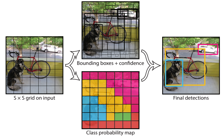
The input is divided into S x S grid

Each grid cell predicts B bounding boxes



5 predictions for one bounding box: x, y, w, h, score

(x, y) center of the box relative to the bounds of grid

w, h are width and height relative to the whole image

the score is a measure of objectness

Each grid cell predicts C conditional class probabilities

Class-specific confidence score is defined as

One predictor is “responsible” for an object having the highest IOU with the ground-truth

The output is an SxSx(Bx5+C) tensor

4.1.3 Experiment Result

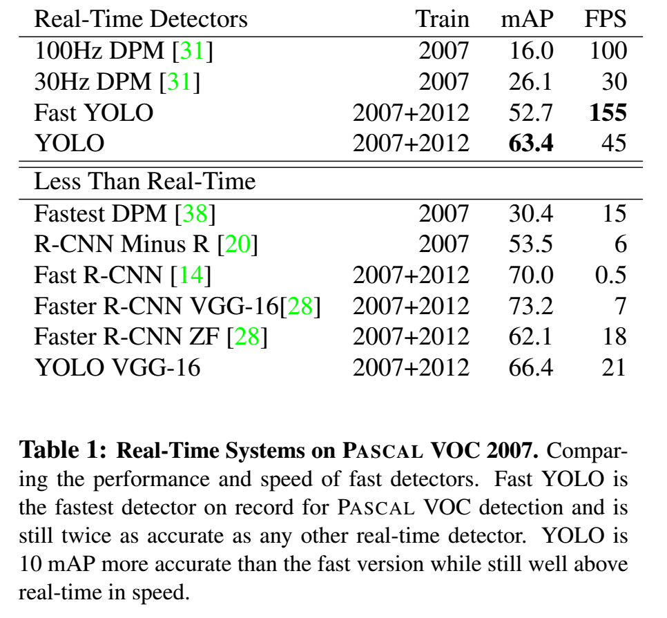
Most effective among real-time detectors

Most efficient among near real-time detectors

4.1.4 Limitations

Too few bounding boxes

Nearby objects

Small objects

Data driven

Sensitive to new or rare ration

4.1.5 Interesting Details – Training

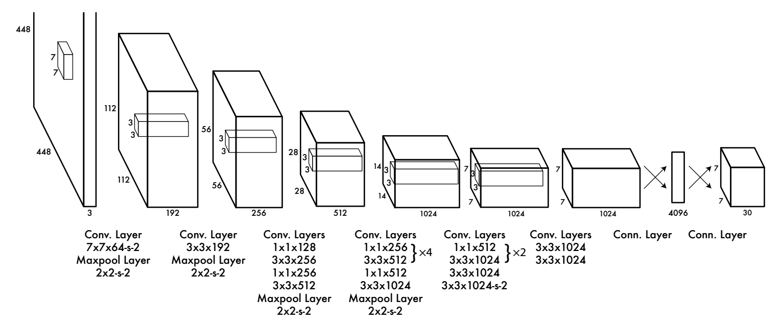
Pre-train the first 20 layers on ImageNet

Pre-train on 224*224 images

Fine-tune 24 layers on detection dataset

Fine-tune on 448*448 images

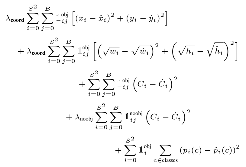
Tricks to balance loss

Weight: localization vs. classification

Weight: positive vs. negative of objectness

Square root: large object vs. small object



“Warm up” to start training

For first epoch, raise 0.001 to 0.01

0.01 for 75 epochs

0.001 for 30 epochs

0.0001 for 30 epochs

4.2 SSD

4.2.1 Single Shot MultiBox Detector

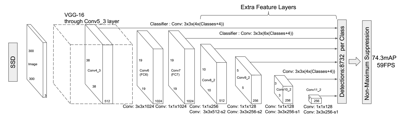
Combine anchor and one-shot prediction

Extract multi-scale features

Refine multi-scale and multi-ratio anchors

Dilated convolution

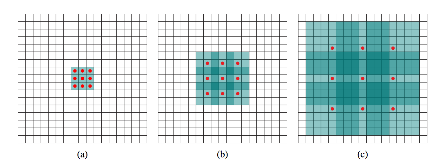
4.2.2 Multi-scale Prediction

Multi-scale and Multi-ratio anchors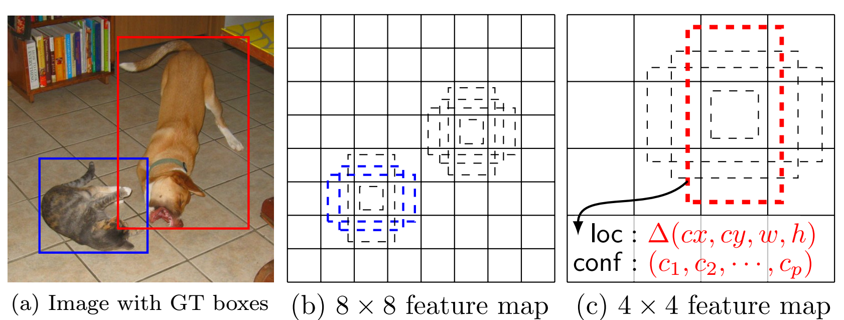



Each feature map cell corresponds to k anchors

Similar to Faster-RCNN, but in multi-scale feature map and directly output category info

Multi-scale feature maps for detection

Additional layers are added to the base network

Different filters are applied to different scale/ratio anchors

(c+4)k filters for k anchors and c categories in one cell, (c+4)kmn outputs for an m*n feature map

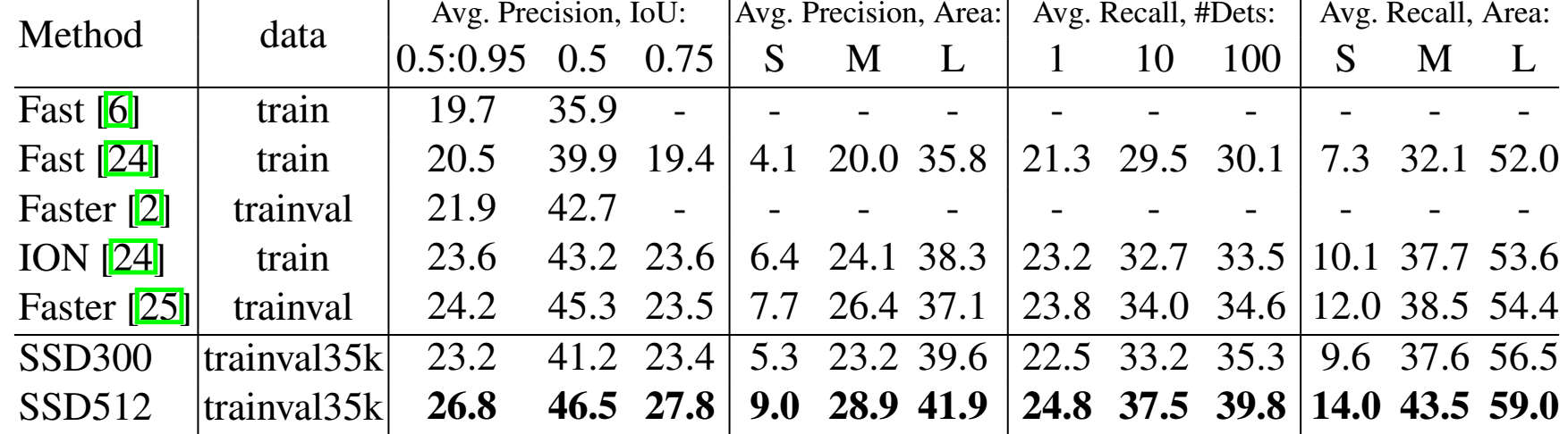
4.2.3 Experiment Result

VOC2012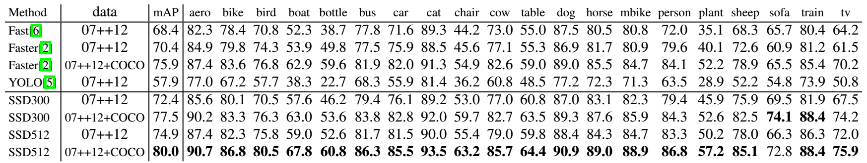



COCO2015

4.2.4 Interesting Details – Training

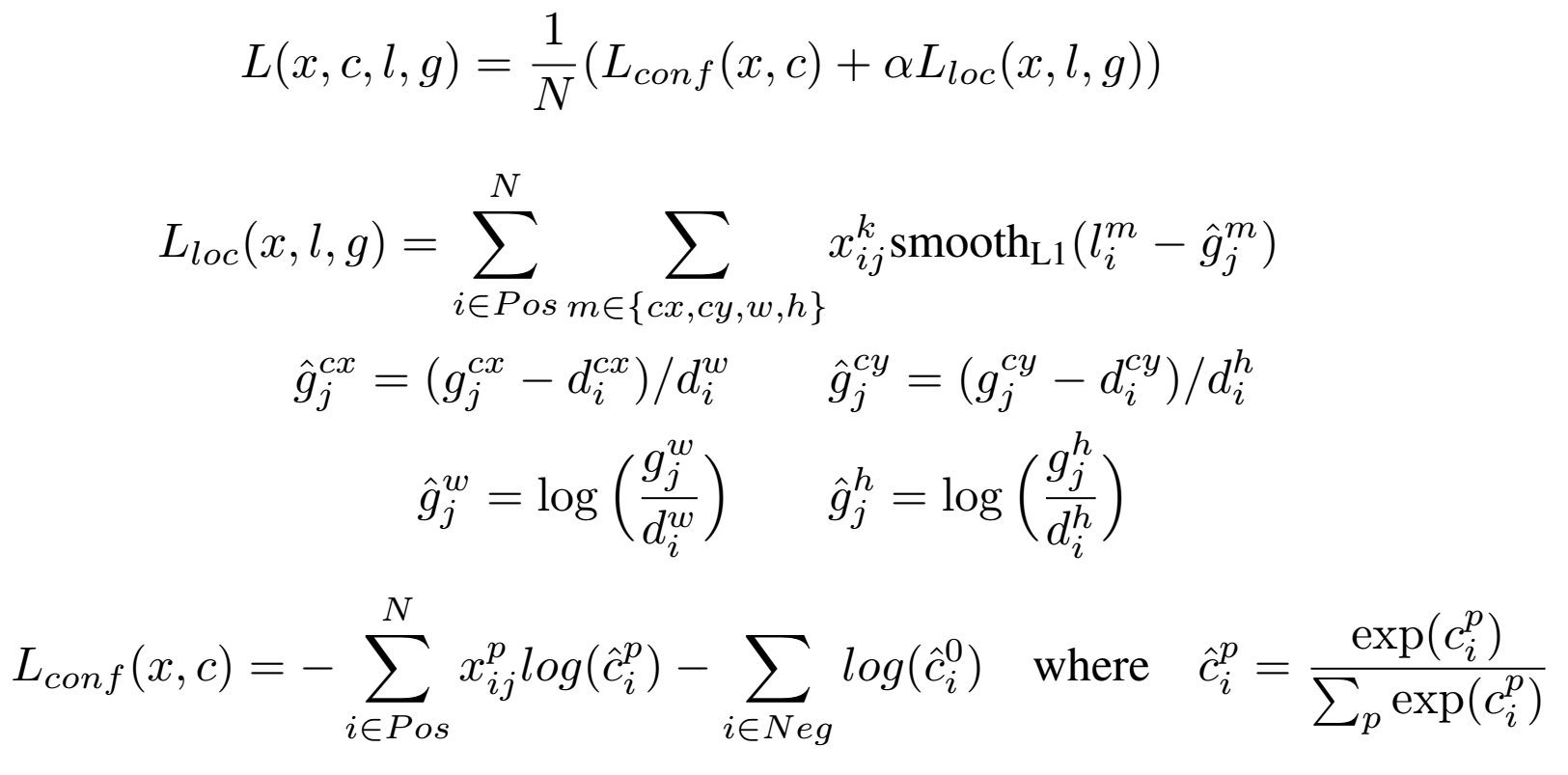
Matching anchors with ground-truth

Match each ground-truth to a default box with the best IOU

Match the anchor to any ground truth with IOU higher than a threshold

Training objective



Scales and aspect ratios for anchors

Regularly spaced scales

{1,2,3,1/2,1/3} – 6 ratios

Hard negative mining

Sort the anchors using the highest confidence loss

Pick the top ones so that neg:pos = 3:1

Data augmentation

Sample randomly from training images

Entire input image

Sample a patch so that min IOU with object is 0.1, 0.3, 0.5, 0.7 or 0.9

Randomly sample a patch, [0.1, 1] of the image, aspect ration [1/2, 2], randomly flip

Comparison

5 Others

PVANET: Deep but Lightweight Neural Networks for Real-time Object Detection (Reading Note)

Variant of Faster-RCNN

Design of architecture

Inside-Outside Net: Detecting Objects in Context with Skip Pooling and Recurrent Neural Networks (Reading Note)

Both local and global information are take into account

Skip pooling uses the information of different scales

R-FCN: Object Detection via Region-based Fully Convolutional Networks (Reading Note)

Position-sensitive RoI pooling

Feature Pyramid Networks for Object Detection (Reading Note)

lateral connections is developed for building high-level semantic feature maps at all scales

Beyond Skip Connections: Top-Down Modulation for Object Detection (Reading Note)

Similar with FPN

YOLO9000: Better, Faster, Stronger (Reading Note)

Better, Faster, Stronger

DSSD: Deconvolutional Single Shot Detector (Reading Note)