时域卷积与频域乘积

转自：http://blog.csdn.net/jacke121/article/details/56668017

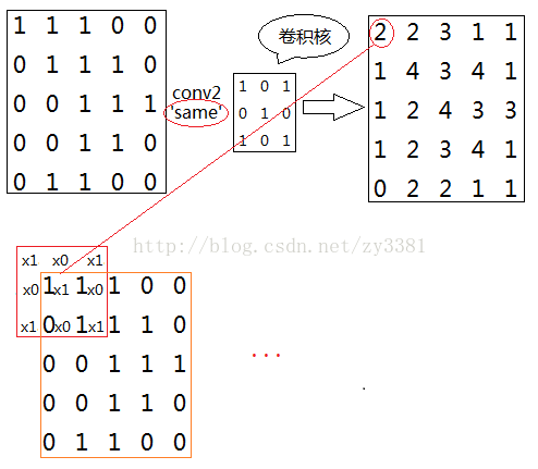
卷积定理：时域的卷积等于频域乘积

情况一，矩阵不拓展：

p=[0,-1,0;-1,4,-1;0,-1,0];%矩阵1

x=magic(5);%矩阵2

a=conv2(x,p,'same');%卷积结果

P=fft2(p,5,5);%矩阵1FFT

X=fft2(x);%矩阵2FFT

aa=X.*P;%频域乘积

r=ifft2(aa);%频域转换

a=

   21    73   -35     2   36

   66   -40    -5    5    13

  -23   -10    0    10    49

   13    -5     5    40  -40

   16    24    61  -47    31

r =

   5.0000   -10.0000        0         60.0000  -55.0000

   10.0000  -5.0000   55.0000  -60.0000   0.0000

  -10.0000   50.0000  -40.0000  -5.0000    5.0000

  45.0000  -45.0000  -10.0000   0.0000   10.0000

  -50.0000   10.0000  -5.0000    5.0000   40.0000

情况二，矩阵拓展：
p=[0,-1,0;-1,4,-1;0,-1,0];%矩阵1

x=magic(5);%矩阵2

a=conv2(x,p,'full');%卷积结果

P=fft2(p,7,7);%矩阵1FFT

X=fft2(x，7，7);%矩阵2FFT

aa=X.*P;%频域乘积

r=ifft2(aa);%频域转换

a=

     0   -17   -24   -1      -8    -15     0

  -17    21    73    -35     2      36   -15

  -23    66  -40    -5       5      13    -16

  -4    -23  -10      0       10    49    -22

  -10   13   -5       5       40   -40    -3

  -11   16    24      61   -47     31    -9

    0   -11  -18     -25   -2     -9        0

r =

  -0.0000  -17.0000  -24.0000   -1.0000  -8.0000  -15.0000   -0.0000

  -17.0000  21.0000   73.0000  -35.0000   2.0000   36.0000  -15.0000

  -23.0000  66.0000  -40.0000   -5.0000   5.0000   13.0000  -16.0000

  -4.0000  -23.0000  -10.0000   -0.0000  10.0000   49.0000  -22.0000

  -10.0000  13.0000   -5.0000    5.0000  40.0000  -40.0000   -3.0000

  -11.0000  16.0000   24.0000   61.0000  -47.0000  31.0000   -9.0000

   0.0000  -11.0000  -18.0000  -25.0000  -2.0000   -9.0000     -0.0000

在处理图像时，所用到的图像复原，都是在时域上做卷积，处理时都是将其转化到频域做乘积，然后再做傅里叶反变换。但是函数在转化成频域时，做傅里叶变化并没有对矩阵扩展。例如图像I为[n,m]大小，掩膜P为[a,b].处理时是将P扩展到[n,m]大小，即fft2（P，a,b）;而不是将I和P都扩展到[n+a-1，m+b-1];经验证，都扩展到[n+a-1，m+b-1]再做频域乘积，在经过傅里叶反变换得到的结果才和时域卷积的结果一致。保持[n,m]大小得到的结果
bcf1
是不对的。例如我上面写道的情况1和情况2，分别对应这两种情况。

掩膜：

    C = conv2(A, B) performs the 2-D convolution of matrices A and B.

    If [ma,na] = size(A), [mb,nb] = size(B), and [mc,nc] = size(C), then

    mc = max([ma+mb-1,ma,mb]) and nc = max([na+nb-1,na,nb]).

 

    C = conv2(H1, H2, A) first convolves each column of A with the vector

    H1 and then convolves each row of the result with the vector H2.  If

    n1 = length(H1), n2 = length(H2), and [mc,nc] = size(C) then

    mc = max([ma+n1-1,ma,n1]) and nc = max([na+n2-1,na,n2]).

    conv2(H1, H2, A) is equivalent to conv2(H1(:)*H2(:).', A) up to

    round-off.

 

    C = conv2(..., SHAPE) returns a subsection of the 2-D

    convolution with size specified by SHAPE:

      'full'  - (default) returns the full 2-D convolution,

      'same'  - returns the central part of the convolution

                that is the same size as A.

      'valid' - returns only those parts of the convolution

                that are computed without the zero-padded edges.

                size(C) = max([ma-max(0,mb-1),na-max(0,nb-1)],0).

关于full, same以及valid三种参数的区别，如下面的实例所示：

[b]full
[/b]



same



valid