机器学习-周志华-个人练习10.6

10.6 试使用MATLAB中的PCA 函数对Yale人脸数据集进行降维，并观察前20个特征向量所对应的图像。

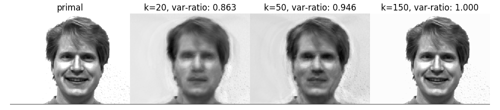
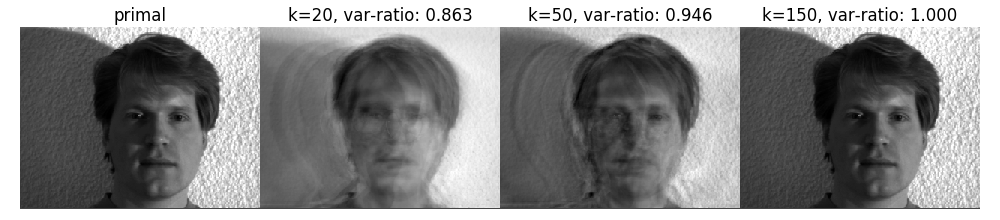
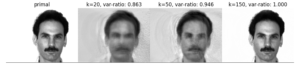
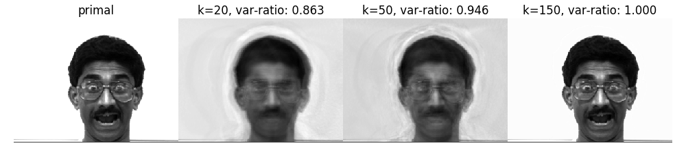
为了便于练习，未使用MATLAB，而是用了scikit-learn.decomposition模块下的PCA进行练习。书上给的Yale人脸数据集访问有点慢（貌似被墙了），我重新上传了一份到百度云（点此下载）。数据集共有样本166个，每张图像的分辨率为320*243（用numpy的shape是倒过来的）。由于图片较多，只选取了几张的PCA（k=20,50,150）的效果进行了展示，具体代码与结果如下，(PCA相关函数的帮助请参考scikit-learn
PCA官方文档)。

由图可见，选取PCA的特征束越多，图像越清晰、明显，而在特征数不足时，会出现大量阴影轮廓，而我们可以用pca.explained_variance_ratio_来查看当前选择的最大k个特征向量的方差占比，方差占比越大则此特征表征的信息越多。

在图中，我们可以发现当k从20增加到150时，选择的k个特征的累计方差占比已经接近于1了（图中为0.9997四舍五入后的结果），而相应地，图像的特征已经与原始图像非常接近了，这意味着我们可以用大约150维的向量来描述一张原本纬数达70000多维的图像，可见PCA在这样的灰度人脸图像下的降维是非常有效的。

# -*- coding: utf-8 -*-
import numpy as np
import scipy.misc as misc
import matplotlib.pyplot as plt
from sklearn.decomposition import PCA
import os

path = 'E:\\...\\yalefaces'
for dirpath, subdir, file_set in os.walk(path):
all_img = [path+'\\'+f for f in file_set] # save the path for all .gif files
m,n = len(all_img), len(misc.imread(all_img[0]).ravel()) # rows and columns of data
data = np.zeros((m,n)) # initializing the data in shape of (m,n)
for i,f in enumerate(all_img):
img = misc.imread(f).ravel() # flatten every 2D img to 1D array
data[i] = img

data_centered = data - data.mean(axis=0) # centering for all samples
data_centered -= data_centered.mean(axis=1).reshape(m, -1) # centering for all attributes
gap = data - data_centered # save the relationship between data and centered one
k = [20,50,150] # set k to be 20,50,100
pca1,pca2,pca3 = PCA(n_components=k[0]),PCA(n_components=k[1]),PCA(n_components=k[2])
r_set,im_set = [],[] # save each pca's variance ratio, output de-centered 1D array
for pca in [pca1,pca2,pca3]:
lower_data = pca.fit_transform(data_centered) # shape=(166,k)
comp = pca.components_ # shape=(k,77760), it's a sparse 2darray
r_set.append(np.sum(pca.explained_variance_ratio_))
im_set.append(np.dot(lower_data, comp) + gap)

fig,[ax0,ax1,ax2,ax3] = plt.subplots(1,4,figsize=(10,2.2))
ax0.imshow(data[1].reshape((243,320)),cmap=plt.cm.gray)
ax0.set_title('primal')
ax0.axis('off')
for i,ax in enumerate([ax1,ax2,ax3]):
ax.imshow(im_set[i][1].reshape((243,320)),cmap=plt.cm.gray)
ax.set_title('k=%s, var-ratio: %.3f' % (k[i], r_set[i]))
ax.axis('off')
plt.subplots_adjust(left=0.02, bottom=0.05, right=0.98, wspace=0)
plt.savefig(r'C:\Users\...\1.png')降维效果如下：