Bagging – building an ensemble of classifers from bootstrap samples
2017-04-24 21:55
483 查看
1. Create a more complex classifcation problem using the
Wine dataset
2. Next encode the class labels into binary format and split the dataset into 60 percent training and 40 percent test set, respectively:
3. Use an unpruned decision tree as the base classifer and create an ensemble of 500 decision trees ftted on different bootstrap samples of the training dataset
4. calculate the accuracy score of the prediction on the training and test dataset to compare the performance of the bagging classifer to the performance of a single unpruned decision tree
Decision tree train/test accuracies 1.000/0.833
5. The substantially lower test accuracy indicates high variance (overftting) of the model
Bagging train/test accuracies 1.000/0.896
6. compare the decision regions between the decision tree and bagging classifer
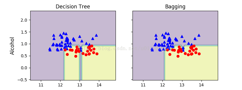
7. Results:
The piece-wise linear decision boundary of the three-node deep decision tree looks smoother in the bagging ensemble
Wine dataset
import pandas as pd
df_wine = pd.read_csv('./datasets/wine/wine.data',
header=None)
# https://archive.ics.uci.edu/ml/machine-learning-databases/wine/wine.data df_wine.columns = ['Class label', 'Alcohol', 'Malic acid', 'Ash',
'Alcalinity of ash', 'Magnesium', 'Total phenols',
'Flavanoids', 'Nonflavanoid phenols', 'Proanthocyanins',
'Color intensity', 'Hue', 'OD280/OD315 of diluted wines',
'Proline']

# drop 1 class
df_wine = df_wine[df_wine['Class label'] != 1]

y = df_wine['Class label'].values
X = df_wine[['Alcohol', 'Hue']].values
2. Next encode the class labels into binary format and split the dataset into 60 percent training and 40 percent test set, respectively:
from sklearn.preprocessing import LabelEncoder
from sklearn.model_selection import train_test_split
le = LabelEncoder()
y = le.fit_transform(y)

X_train, X_test, y_train, y_test =\
train_test_split(X, y,
test_size=0.40,
random_state=1)
3. Use an unpruned decision tree as the base classifer and create an ensemble of 500 decision trees ftted on different bootstrap samples of the training dataset
from sklearn.ensemble import BaggingClassifier
tree = DecisionTreeClassifier(criterion='entropy',
max_depth=None,
random_state=1)

bag = BaggingClassifier(base_estimator=tree,
n_estimators=500,
max_samples=1.0,
max_features=1.0,
bootstrap=True,
bootstrap_features=False,
n_jobs=1,
random_state=1)
4. calculate the accuracy score of the prediction on the training and test dataset to compare the performance of the bagging classifer to the performance of a single unpruned decision tree
from sklearn.metrics import accuracy_score
tree = tree.fit(X_train, y_train)
y_train_pred = tree.predict(X_train)
y_test_pred = tree.predict(X_test)

tree_train = accuracy_score(y_train, y_train_pred)
tree_test = accuracy_score(y_test, y_test_pred)
print('Decision tree train/test accuracies %.3f/%.3f'
% (tree_train, tree_test))
Decision tree train/test accuracies 1.000/0.833
5. The substantially lower test accuracy indicates high variance (overftting) of the model
bag = bag.fit(X_train, y_train)
y_train_pred = bag.predict(X_train)
y_test_pred = bag.predict(X_test)

bag_train = accuracy_score(y_train, y_train_pred)
bag_test = accuracy_score(y_test, y_test_pred)
print('Bagging train/test accuracies %.3f/%.3f'
% (bag_train, bag_test))
Bagging train/test accuracies 1.000/0.896
6. compare the decision regions between the decision tree and bagging classifer
x_min = X_train[:, 0].min() - 1
x_max = X_train[:, 0].max() + 1
y_min = X_train[:, 1].min() - 1
y_max = X_train[:, 1].max() + 1

xx, yy = np.meshgrid(np.arange(x_min, x_max, 0.1),
np.arange(y_min, y_max, 0.1))

f, axarr = plt.subplots(nrows=1, ncols=2,
sharex='col',
sharey='row',
figsize=(8, 3))

for idx, clf, tt in zip([0, 1],
[tree, bag],
['Decision Tree', 'Bagging']):
clf.fit(X_train, y_train)

Z = clf.predict(np.c_[xx.ravel(), yy.ravel()])
Z = Z.reshape(xx.shape)

axarr[idx].contourf(xx, yy, Z, alpha=0.3)
axarr[idx].scatter(X_train[y_train == 0, 0],
X_train[y_train == 0, 1],
c='blue', marker='^')

axarr[idx].scatter(X_train[y_train == 1, 0],
X_train[y_train == 1, 1],
c='red', marker='o')

axarr[idx].set_title(tt)

axarr[0].set_ylabel('Alcohol', fontsize=12)
plt.text(10.2, -1.2,
s='Hue',
ha='center', va='center', fontsize=12)
plt.show()
7. Results:
The piece-wise linear decision boundary of the three-node deep decision tree looks smoother in the bagging ensemble

相关文章推荐
- startActivity时报错Calling startActivity() from outside of an Activity context requires the FLAG_ACTIVI
- Caused by: android.util.AndroidRuntimeException: Calling startActivity() from outside of an Activity
- Calling startActivity() from outside of an Activity
- The problem of waiting time when launching a unix shell command from an application engine
- android.util.AndroidRuntimeException: Calling startActivity() from outside of an Activity
- Caused by: android.util.AndroidRuntimeException: Calling startActivity() from outside of an Activity
- Caused by: android.util.AndroidRuntimeException: Calling startActivity() from outside of an Activity
- Android - Error:Calling startActivity() from outside of an activity context
- How To Retrieve the URL of a Web Page from an ActiveX Control
- 【论文笔记】One Millisecond Face Alignment with an Ensemble of Regression Trees
- context.startActivity时报错startActivity() from outside of an Activity context require the FLAG_ACTIVITY_NEW_TASK flag
- android.util.AndroidRuntimeException: Calling startActivity() from outside of an Activity
- C++之invalid initialization of non-const reference of type ‘int&’ from an rvalue of type ‘int’
- Android—android.util.AndroidRuntimeException: Calling startActivity() from outside of an Activity
- android.util.AndroidRuntimeException: Calling startActivity from outside of an Activity context
- Calling startActivity() from outside of an Activity context requires the FLAG_ACTIVITY_NEW_TASK flag
- Calling startActivity() from outside of an Activity
- identifier of an instance was altered from XXXX to XXXX解决
- org.hibernate.HibernateException: identifier of an instance of XXX was altered from X to X
- LSCTableView: Building an Open, Drop-in Replacement of UITableView