Computer Vision for Predicting Facial Attractiveness

转载：http://www.learnopencv.com/computer-vision-for-predicting-facial-attractiveness/

Computer Vision for Predicting Facial Attractiveness

JULY 27, 2015 BY AVI SINGH 13 COMMENTS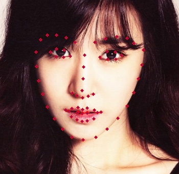

Most of us have looked in the mirror and wondered how good we look. But, it is often difficult to be objective while judging our own attractiveness, and we are often too embarrassed to ask for others’ opinion. What if there was a computer program that could answer this question for you, without a human to look at your image? Pretty nifty, huh?In this post, I will show you how we can use computer vision and machine learning to predict facial attractiveness of an individual from a single photograph. I will use OpenCV, Numpy and scikit-learn to develop a completely automated pipeline that takes a photograph of a person’s face, and rates the photo on a scale of 1 to 5. The code is available at the bottom of this page.This is a guest post by Avi Singh — an undergraduate student at Indian Institute of Technology, Kanpur. Visit his page to see all the cool projects he has done.While applying machine learning algorithms to a computer vision problems, the high dimensionality of visual data presents a huge challenge. Even a relatively low-res 200×200 image translates to a feature vector of length 40,000. Deep learning models like Convolutional Neural Nets can work directly with raw images, but they require huge amounts of data to be successful. Since we only have a access to a small-ish dataset in this tutorial (500 images), we cannot work with raw images, and we therefore need to extract some informative features from these images.

Feature Extraction for Facial Attractiveness

One feature that determines facial attractiveness (as cited in psychology literature), is the ratio of the distances between the various facial landmarks. Facial landmarks are features like the corner of the eyes, tip of the nose, lowest point on the chin, etc. You can see these points marked in red on the image at the top of this page. In order to calculate these ratios, we would need to have an algorithm with can localize the landmarks accurately in an image. In this post, we would be making use of an open-source software called the CLM framework to extract these landmarks. It is written in C++, and utilizes OpenCV 3.0. It has instructions for both Windows and Ubuntu (which should also work with OS X without much change), and works out of the box. If you do not want to bother with setting up this piece of software, I will be providing a file with facial landmark coordinates of all the images that I use in this tutorial, and you can then tinker with the Machine Learning part of the pipeline.

Facial Attractiveness Dataset

Now that we have a way to extract features, what we need now is the data to extract these features from. While  there are several datasets available to benchmark facial attractiveness, most of them require signing up, and won’t be available to people outside the academia. However, I was able to find one dataset that does not have these requirements. It is called the SCUT-FBP dataset, and contains images of 500 Asian females. Each image is rated by 10 users, and we would be attempting to predict the average rating for each image.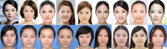

Generating Features

We first run the CLM-framework on these images and write the facial landmarks to a file. Click here to get the file. Next we use a python script to calculate ratios between all possible pairs of points, and save the results to a text file. Now that we have our features, we can finally delve into Machine Learning!

Machine Learning for Rating a Face

While there are numerous packages available for Machine Learning, I chose to go with scikit-learn in this post because it’s easy to install and use. Installing scikit-learn is as simple as:UbuntuMac OSXWindowsFor more details, you can visit the official scikit-learn installation page.Once you are past the installation, you will notice that working with scikit-learn is a walk in the park. Follow these instructions to load the data (both features and ratings):Now, if you open the features file, you will see that the number of features per image are extremely large (for the size of our dataset), and if we directly use them, we will face a problem called the Curse of Dimensionality. What we need is to project this large feature space into a smaller feature space, and the algorithm to do so is Principal Component Analysis (PCA). Using PCA in scikit-learn is pretty simple, and the following code is all you need:In the above code, n_components is a hyper-parameter, and it’s value can be chosen by testing the performance of the model on a validation set (or cross-validation).Now we need to choose what model we should use for our problem. Our problem is a regression problem. There are several models/algorithms available to deal with these problem like Linear Regression, Support Vector Regressors (SVR), Random Forest Regression, Gaussian Process Regression, et all.Let’s have a look at the code that we need to train a linear model:The above code will fit a linear regressor on the traininng set, and then store the predictions. The next step in our pipeline is to do performance evaluation. One way to do so is to calculate the Pearson correlation between the predicted ratings and the actual ratings. This can be calculated using Numpy as shown below

Results

One thing that I have not talked about so far is how I split the dataset into training and testing. To get the initial results, I used a split of 450 training images and 50 testing images. But, since we have very limited data, we should try to make use of as much data as possible to train the model. One way to do so is leave-one-out cross-validation. In this technique, we take 499 images for training, and then test the model on the one image that we left out. We do this for all 500 images (train 500 models), and then calculate the Pearson correlation between the predictions and the actual ratings. The graphic below highlights the performance obtained when I evaluated several models using this method.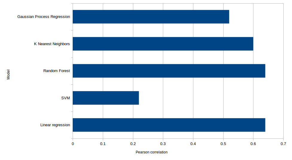



Linear Regression and Random Forest perform the best, with a Pearson correlation of 0.64 each. K-Nearest Neighbors is comparable with 0.6, while Gaussian Process regression lags a bit at 0.52. SVM perform really poorly, which was somewhat of a surprise for me.

Testing on Celebrities

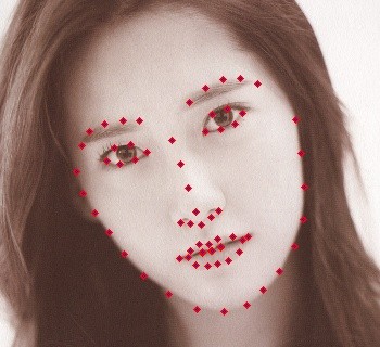
Yoona, Predicted Rating: 3.6

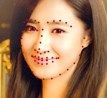
Yuri, Predicted Rating: 3.4

Tiffany, Predicted Rating: 3.8Now, let us have some fun, and use the model that we just trained on some celebrity photographs! I am personally a fan of the K-pop group Girls’ Generation, and since the training images in the dataset are all asian females, the singers of Girls’ Generations are ideal for our experiment!As one might expect, the predicted ratings are quite high (the average was 2.7 in the training set). This shows that the algorithms generalizes well, at least for faces of the same gender and ethnicity.There are a lot of things that we could do to improve the performance. The present algorithm takes into account only the shape of the face. Some other important features might be skin gradients and hair style, which I have not modeled in this blog post. Perhaps a future approach can use pre-trained Convolutional Neural Nets to extract high level features, and then something like an Random Forest or an SVM at the top can do the regression.

Subscribe & Download Code

You can download the code for this article on GitHub. To get access to all code and images used in all articles ( including this one ), please subscribeto our newsletter. You will also receive a free Computer Vision Resource guide. In our newsletter we share OpenCV tutorials and examples written in C++/Python, and Computer Vision and Machine Learning algorithms and news.