加速器陀螺仪基本原理
2017-03-24 09:55
453 查看
转自:http://www.instructables.com/id/Accelerometer-Gyro-Tutorial/
非常简单清晰明了的一片介绍文章
This guide is intended to everyone interested in in using Accelerometers and Gyroscopes as well as combination IMU devices (Inertial
Measurement Unit) in their electronics projects
We'll cover:
What does an accelerometer measure?
What does a gyroscope (aka gyro) measure?
How to convert analog-to-digital (ADC) readings that you get from these sensor to physical units (those would be g for accelerometer, deg/s for gyroscope)
How to combine accelerometer and gyroscope readings in order to obtain accurate information about the inclination of your device relative to the ground plane
Throughout the article I will try to keep the math to the minimum. If you know what Sine/Cosine/Tangent are then you should be able to understand and use these ideas in your project no matter what
platform you're using: Arduino, Propeller, Basic Stamp, Atmel chips, Microchip PIC, etc.
There are people out there who believe that you need complex math in order to make use of an IMU unit (complex FIR or IIR filters such as Kalman filters, Parks-McClellan filters, etc). You can research all those and achieve wonderful but complex results. My
way of explaining things require just basic math. I am a great believer in simplicity. I think a system that is simple is easier to control and monitor, besides many embedded devices do not have the power and resources to implement complex algorithms requiring
matrix calculations.
I'll use as an example a new IMU unit, the Acc_Gyro
Accelerometer + Gyro IMU. We'll use parameters of this device in our examples below. This unit is a good device to start with because it consists of 2 devices:
- LIS331AL (data sheet) - a triaxial
2G accelerometer
- LPR550AL (data sheet) - a dual-axis pitch and roll, 500 deg/sec gyroscope
Together they represent a 5-Degrees of Freedom Inertial Measurement Unit. Now that's a fancy name! Nevertheless, behind the fancy name is a very useful combination device that we'll cover and explain
in detail in this guide.
Step 1: The Accelerometer

To understand this unit we'll start with the accelerometer. When thinking about accelerometers it is often useful to image a box in shape of a cube with a ball inside it. You may imagine something else like a cookie or a donut , but I'll imagine a ball:
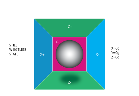
If we take this box in a place with no gravitation fields or for that matter with no other fields that might affect the ball's position - the ball will simply float in the middle of the box. You can imagine the
box is in outer-space far-far away from any cosmic bodies, or if such a place is hard to find imagine at least a space craft orbiting around the planet where everything is in weightless state . From the picture above you can see that we assign to each axis
a pair of walls (we removed the wall Y+ so we can look inside the box). Imagine that each wall is pressure sensitive. If we move suddenly the box to the left (we accelerate it with acceleration 1g = 9.8m/s^2), the ball will hit the wall X-. We then measure
the pressure force that the ball applies to the wall and output a value of -1g on the X axis.
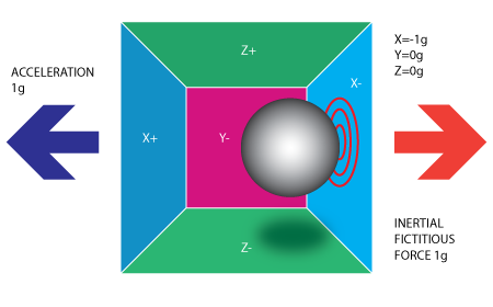
Please note that the accelerometer will actually detect a force that is directed in the opposite direction from the acceleration vector. This force is often called Inertial
Force or Fictitious Force . One thing you should learn from this is that an accelerometer measures acceleration indirectly through a force that is applied to one of it's walls (according to our model, it might be a spring or something else in real life
accelerometers). This force can be caused by the acceleration , but as we'll see in the next example it is not always caused by acceleration.
If we take our model and put it on Earth the ball will fall on the Z- wall and will apply a force of 1g on the bottom wall, as shown in the picture below:

In this case the box isn't moving but we still get a reading of -1g on the Z axis. The pressure that the ball has applied on the wall was caused by a gravitation force. In theory it could be a different type of
force - for example, if you imagine that our ball is metallic, placing a magnet next to the box could move the ball so it hits another wall. This was said just to prove that in essence accelerometer measures force not acceleration. It just happens that acceleration
causes an inertial force that is captured by the force detection mechanism of the accelerometer.
While this model is not exactly how a MEMS sensor is constructed it is often useful in solving accelerometer related problems. There are actually similar sensors that have metallic balls inside, they are called
tilt switches, however they are more primitive and usually they can only tell if the device is inclined within some range or not, not the extent of inclination.
So far we have analyzed the accelerometer output on a single axis and this is all you'll get with a single axis accelerometers. The real value of triaxial accelerometers comes from the fact that they can detect
inertial forces on all three axes. Let's go back to our box model, and let's rotate the box 45 degrees to the right. The ball will touch 2 walls now: Z- and X- as shown in the picture below:
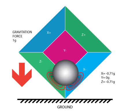
The values of 0.71 are not arbitrary, they are actually an approximation for SQRT(1/2). This will become more clear as we introduce our next model for the accelerometer.
In the previous model we have fixed the gravitation force and rotated our imaginary box. In last 2 examples we have analyzed the output in 2 different box positions, while the force vector remained constant. While
this was useful in understanding how the accelerometer interacts with outside forces, it is more practical to perform calculations if we fix the coordinate system to the axes of the accelerometer and imagine that the force vector rotates around us.
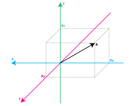
Please have a look at the model above, I preserved the colors of the axes so you can make a mental transition from the previous model to the new one. Just imagine that each axis in the new model is perpendicular
to the respective faces of the box in the previous model. The vector R is the force vector that the accelerometer is measuring (it could be either the gravitation force or the inertial force from the examples above or a combination of both). Rx, Ry, Rz are
projection of the R vector on the X,Y,Z axes. Please notice the following relation:
R^2 = Rx^2 + Ry^2 + Rz^2 (Eq. 1)
which is basically the equivalent of the Pythagorean theorem in 3D.
Remember that a little bit earlier I told you that the values of SQRT(1/2) ~ 0.71 are not random. If you plug them in the formula above, after recalling that our gravitation force was 1 g we can verify that:
1^2 = (-SQRT(1/2) )^2 + 0 ^2 + (-SQRT(1/2))^2
simply by substituting R=1, Rx = -SQRT(1/2), Ry = 0 , Rz = -SQRT(1/2) in Eq.1
After a long preamble of theory we're getting closer to real life accelerometers. The values Rx, Ry, Rz are actually linearly related to the values that your real-life accelerometer will output and that you can
use for performing various calculations.
Before we get there let's talk a little about the way accelerometers will deliver this information to us. Most accelerometers will fall in two categories: digital and analog. Digital accelerometers will give you
information using a serial protocol like I2C , SPI or USART, while analog accelerometers will output a voltage level within a predefined range that you have to convert to a digital value using an ADC (analog to digital converter) module. I will not go into
much detail about how ADC works, partly because it is such an extensive topic and partly because it is different from one platform to another. Some microcontroller will have a built-in ADC modules some of them will need external components in order to perform
the ADC conversions. No matter what type of ADC module you use you'll end up with a value in a certain range. For example a 10-bit ADC module will output a value in the range of 0..1023, note that 1023 = 2^10 -1. A 12-bit ADC module will output a value in
the range of 0..4095, note that 4095 = 2^12-1.
Let's move on by considering a simple example, suppose our 10bit ADC module gave us the following values for the three accelerometer channels (axes):
AdcRx = 586
AdcRy = 630
AdcRz = 561
Each ADC module will have a reference voltage, let's assume in our example it is 3.3V. To convert a 10bit adc value to voltage we use the following formula:
VoltsRx = AdcRx * Vref / 1023
A quick note here: that for 8bit ADC the last divider would be 255 = 2 ^ 8 -1 , and for 12bit ADC last divider would be 4095 = 2^12 -1.
Applying this formula to all 3 channels we get:
VoltsRx = 586 * 3.3V / 1023 =~ 1.89V (we round all results to 2 decimal points)
VoltsRy = 630 * 3.3V / 1023 =~ 2.03V
VoltsRz = 561 * 3.3V / 1023 =~ 1.81V
Each accelerometer has a zero-g voltage level, you can find it in specs, this is the voltage that corresponds to 0g. To get a signed voltage value we need to calculate the shift from this level. Let's say our 0g
voltage level is VzeroG = 1.65V. We calculate the voltage shifts from zero-g voltage as follows::
DeltaVoltsRx = 1.89V - 1.65V = 0.24V
DeltaVoltsRy = 2.03V - 1.65V = 0.38V
DeltaVoltsRz = 1.81V - 1.65V = 0.16V
We now have our accelerometer readings in Volts , it's still not in g (9.8 m/s^2), to do the final conversion we apply the accelerometer sensitivity, usually expressed in mV/g. Lets say our Sensitivity = 478.5mV/g
= 0.4785V/g. Sensitivity values can be found in accelerometer specifications. To get the final force values expressed in g we use the following formula:
Rx = DeltaVoltsRx / Sensitivity
Rx = 0.24V / 0.4785V/g =~ 0.5g
Ry = 0.38V / 0.4785V/g =~ 0.79g
Rz = 0.16V / 0.4785V/g =~ 0.33g
We could of course combine all steps in one formula, but I went through all the steps to make it clear how you go from ADC readings to a force vector component expressed in g.
Rx = (AdcRx * Vref / 1023 - VzeroG) / Sensitivity
(Eq.2)
Ry = (AdcRy * Vref / 1023 - VzeroG) / Sensitivity
Rz = (AdcRz * Vref / 1023 - VzeroG) / Sensitivity
We now have all 3 components that define our inertial force vector, if the device is not subject to other forces other than gravitation, we can assume this is the direction of our gravitation force vector. If you
want to calculate inclination of device relative to the ground you can calculate the angle between this vector and Z axis. If you are also interested in per-axis direction of inclination you can split this result into 2 components: inclination on the X and
Y axis that can be calculated as the angle between gravitation vector and X / Y axes. Calculating these angles is more simple than you might think, now that we have calculated the values for Rx,Ry and Rz. Let's go back to our last accelerometer model and do
some additional notations:
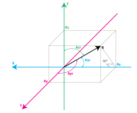
The angles that we are interested in are the angles between X,Y,Z axes and the force vector R. We'll define these angles as Axr, Ayr, Azr. You can notice from the right-angle triangle formed by R and Rx that:
cos(Axr) = Rx / R , and similarly :
cos(Ayr) = Ry / R
cos(Azr) = Rz / R
We can deduct from Eq.1 that R = SQRT( Rx^2 + Ry^2 + Rz^2).
We can find now our angles by using arccos() function (the inverse cos() function ):
Axr = arccos(Rx/R)
Ayr = arccos(Ry/R)
Azr = arccos(Rz/R)
We've gone a long way to explain the accelerometer model, just to come up to these formulas. Depending on your applications you might want to use any intermediate formulas that we have derived. We'll also introduce
the gyroscope model soon, and we'll see how accelerometer and gyroscope data can be combined to provide even more accurate inclination estimations.
But before we do that let's do some more useful notations:
cosX = cos(Axr) = Rx / R
cosY = cos(Ayr) = Ry / R
cosZ = cos(Azr) = Rz / R
This triplet is often called Direction Cosine , and it basically represents
the unit vector (vector with length 1) that has same direction as our R vector. You can easily verify that:
SQRT(cosX^2 + cosY^2 + cosZ^2) = 1
This is a nice property since it absolve us from monitoring the modulus(length) of R vector. Often times if we're just interested in direction of our inertial vector, it makes sense to normalize it's modulus in
order to simplify other calculations.
非常简单清晰明了的一片介绍文章
Introduction
This guide is intended to everyone interested in in using Accelerometers and Gyroscopes as well as combination IMU devices (InertialMeasurement Unit) in their electronics projects
We'll cover:
What does an accelerometer measure?
What does a gyroscope (aka gyro) measure?
How to convert analog-to-digital (ADC) readings that you get from these sensor to physical units (those would be g for accelerometer, deg/s for gyroscope)
How to combine accelerometer and gyroscope readings in order to obtain accurate information about the inclination of your device relative to the ground plane
Throughout the article I will try to keep the math to the minimum. If you know what Sine/Cosine/Tangent are then you should be able to understand and use these ideas in your project no matter what
platform you're using: Arduino, Propeller, Basic Stamp, Atmel chips, Microchip PIC, etc.
There are people out there who believe that you need complex math in order to make use of an IMU unit (complex FIR or IIR filters such as Kalman filters, Parks-McClellan filters, etc). You can research all those and achieve wonderful but complex results. My
way of explaining things require just basic math. I am a great believer in simplicity. I think a system that is simple is easier to control and monitor, besides many embedded devices do not have the power and resources to implement complex algorithms requiring
matrix calculations.
I'll use as an example a new IMU unit, the Acc_Gyro
Accelerometer + Gyro IMU. We'll use parameters of this device in our examples below. This unit is a good device to start with because it consists of 2 devices:
- LIS331AL (data sheet) - a triaxial
2G accelerometer
- LPR550AL (data sheet) - a dual-axis pitch and roll, 500 deg/sec gyroscope
Together they represent a 5-Degrees of Freedom Inertial Measurement Unit. Now that's a fancy name! Nevertheless, behind the fancy name is a very useful combination device that we'll cover and explain
in detail in this guide.
Step 1: The Accelerometer
To understand this unit we'll start with the accelerometer. When thinking about accelerometers it is often useful to image a box in shape of a cube with a ball inside it. You may imagine something else like a cookie or a donut , but I'll imagine a ball:
If we take this box in a place with no gravitation fields or for that matter with no other fields that might affect the ball's position - the ball will simply float in the middle of the box. You can imagine the
box is in outer-space far-far away from any cosmic bodies, or if such a place is hard to find imagine at least a space craft orbiting around the planet where everything is in weightless state . From the picture above you can see that we assign to each axis
a pair of walls (we removed the wall Y+ so we can look inside the box). Imagine that each wall is pressure sensitive. If we move suddenly the box to the left (we accelerate it with acceleration 1g = 9.8m/s^2), the ball will hit the wall X-. We then measure
the pressure force that the ball applies to the wall and output a value of -1g on the X axis.
Please note that the accelerometer will actually detect a force that is directed in the opposite direction from the acceleration vector. This force is often called Inertial
Force or Fictitious Force . One thing you should learn from this is that an accelerometer measures acceleration indirectly through a force that is applied to one of it's walls (according to our model, it might be a spring or something else in real life
accelerometers). This force can be caused by the acceleration , but as we'll see in the next example it is not always caused by acceleration.
If we take our model and put it on Earth the ball will fall on the Z- wall and will apply a force of 1g on the bottom wall, as shown in the picture below:
In this case the box isn't moving but we still get a reading of -1g on the Z axis. The pressure that the ball has applied on the wall was caused by a gravitation force. In theory it could be a different type of
force - for example, if you imagine that our ball is metallic, placing a magnet next to the box could move the ball so it hits another wall. This was said just to prove that in essence accelerometer measures force not acceleration. It just happens that acceleration
causes an inertial force that is captured by the force detection mechanism of the accelerometer.
While this model is not exactly how a MEMS sensor is constructed it is often useful in solving accelerometer related problems. There are actually similar sensors that have metallic balls inside, they are called
tilt switches, however they are more primitive and usually they can only tell if the device is inclined within some range or not, not the extent of inclination.
So far we have analyzed the accelerometer output on a single axis and this is all you'll get with a single axis accelerometers. The real value of triaxial accelerometers comes from the fact that they can detect
inertial forces on all three axes. Let's go back to our box model, and let's rotate the box 45 degrees to the right. The ball will touch 2 walls now: Z- and X- as shown in the picture below:
The values of 0.71 are not arbitrary, they are actually an approximation for SQRT(1/2). This will become more clear as we introduce our next model for the accelerometer.
In the previous model we have fixed the gravitation force and rotated our imaginary box. In last 2 examples we have analyzed the output in 2 different box positions, while the force vector remained constant. While
this was useful in understanding how the accelerometer interacts with outside forces, it is more practical to perform calculations if we fix the coordinate system to the axes of the accelerometer and imagine that the force vector rotates around us.
Please have a look at the model above, I preserved the colors of the axes so you can make a mental transition from the previous model to the new one. Just imagine that each axis in the new model is perpendicular
to the respective faces of the box in the previous model. The vector R is the force vector that the accelerometer is measuring (it could be either the gravitation force or the inertial force from the examples above or a combination of both). Rx, Ry, Rz are
projection of the R vector on the X,Y,Z axes. Please notice the following relation:
R^2 = Rx^2 + Ry^2 + Rz^2 (Eq. 1)
which is basically the equivalent of the Pythagorean theorem in 3D.
Remember that a little bit earlier I told you that the values of SQRT(1/2) ~ 0.71 are not random. If you plug them in the formula above, after recalling that our gravitation force was 1 g we can verify that:
1^2 = (-SQRT(1/2) )^2 + 0 ^2 + (-SQRT(1/2))^2
simply by substituting R=1, Rx = -SQRT(1/2), Ry = 0 , Rz = -SQRT(1/2) in Eq.1
After a long preamble of theory we're getting closer to real life accelerometers. The values Rx, Ry, Rz are actually linearly related to the values that your real-life accelerometer will output and that you can
use for performing various calculations.
Before we get there let's talk a little about the way accelerometers will deliver this information to us. Most accelerometers will fall in two categories: digital and analog. Digital accelerometers will give you
information using a serial protocol like I2C , SPI or USART, while analog accelerometers will output a voltage level within a predefined range that you have to convert to a digital value using an ADC (analog to digital converter) module. I will not go into
much detail about how ADC works, partly because it is such an extensive topic and partly because it is different from one platform to another. Some microcontroller will have a built-in ADC modules some of them will need external components in order to perform
the ADC conversions. No matter what type of ADC module you use you'll end up with a value in a certain range. For example a 10-bit ADC module will output a value in the range of 0..1023, note that 1023 = 2^10 -1. A 12-bit ADC module will output a value in
the range of 0..4095, note that 4095 = 2^12-1.
Let's move on by considering a simple example, suppose our 10bit ADC module gave us the following values for the three accelerometer channels (axes):
AdcRx = 586
AdcRy = 630
AdcRz = 561
Each ADC module will have a reference voltage, let's assume in our example it is 3.3V. To convert a 10bit adc value to voltage we use the following formula:
VoltsRx = AdcRx * Vref / 1023
A quick note here: that for 8bit ADC the last divider would be 255 = 2 ^ 8 -1 , and for 12bit ADC last divider would be 4095 = 2^12 -1.
Applying this formula to all 3 channels we get:
VoltsRx = 586 * 3.3V / 1023 =~ 1.89V (we round all results to 2 decimal points)
VoltsRy = 630 * 3.3V / 1023 =~ 2.03V
VoltsRz = 561 * 3.3V / 1023 =~ 1.81V
Each accelerometer has a zero-g voltage level, you can find it in specs, this is the voltage that corresponds to 0g. To get a signed voltage value we need to calculate the shift from this level. Let's say our 0g
voltage level is VzeroG = 1.65V. We calculate the voltage shifts from zero-g voltage as follows::
DeltaVoltsRx = 1.89V - 1.65V = 0.24V
DeltaVoltsRy = 2.03V - 1.65V = 0.38V
DeltaVoltsRz = 1.81V - 1.65V = 0.16V
We now have our accelerometer readings in Volts , it's still not in g (9.8 m/s^2), to do the final conversion we apply the accelerometer sensitivity, usually expressed in mV/g. Lets say our Sensitivity = 478.5mV/g
= 0.4785V/g. Sensitivity values can be found in accelerometer specifications. To get the final force values expressed in g we use the following formula:
Rx = DeltaVoltsRx / Sensitivity
Rx = 0.24V / 0.4785V/g =~ 0.5g
Ry = 0.38V / 0.4785V/g =~ 0.79g
Rz = 0.16V / 0.4785V/g =~ 0.33g
We could of course combine all steps in one formula, but I went through all the steps to make it clear how you go from ADC readings to a force vector component expressed in g.
Rx = (AdcRx * Vref / 1023 - VzeroG) / Sensitivity
(Eq.2)
Ry = (AdcRy * Vref / 1023 - VzeroG) / Sensitivity
Rz = (AdcRz * Vref / 1023 - VzeroG) / Sensitivity
We now have all 3 components that define our inertial force vector, if the device is not subject to other forces other than gravitation, we can assume this is the direction of our gravitation force vector. If you
want to calculate inclination of device relative to the ground you can calculate the angle between this vector and Z axis. If you are also interested in per-axis direction of inclination you can split this result into 2 components: inclination on the X and
Y axis that can be calculated as the angle between gravitation vector and X / Y axes. Calculating these angles is more simple than you might think, now that we have calculated the values for Rx,Ry and Rz. Let's go back to our last accelerometer model and do
some additional notations:
The angles that we are interested in are the angles between X,Y,Z axes and the force vector R. We'll define these angles as Axr, Ayr, Azr. You can notice from the right-angle triangle formed by R and Rx that:
cos(Axr) = Rx / R , and similarly :
cos(Ayr) = Ry / R
cos(Azr) = Rz / R
We can deduct from Eq.1 that R = SQRT( Rx^2 + Ry^2 + Rz^2).
We can find now our angles by using arccos() function (the inverse cos() function ):
Axr = arccos(Rx/R)
Ayr = arccos(Ry/R)
Azr = arccos(Rz/R)
We've gone a long way to explain the accelerometer model, just to come up to these formulas. Depending on your applications you might want to use any intermediate formulas that we have derived. We'll also introduce
the gyroscope model soon, and we'll see how accelerometer and gyroscope data can be combined to provide even more accurate inclination estimations.
But before we do that let's do some more useful notations:
cosX = cos(Axr) = Rx / R
cosY = cos(Ayr) = Ry / R
cosZ = cos(Azr) = Rz / R
This triplet is often called Direction Cosine , and it basically represents
the unit vector (vector with length 1) that has same direction as our R vector. You can easily verify that:
SQRT(cosX^2 + cosY^2 + cosZ^2) = 1
This is a nice property since it absolve us from monitoring the modulus(length) of R vector. Often times if we're just interested in direction of our inertial vector, it makes sense to normalize it's modulus in
order to simplify other calculations.

相关文章推荐
- 加速器,陀螺仪测量移动距离的方法
- 加速器,陀螺仪测量移动距离的方法
- 21.0~21.5 加速器与陀螺仪 Core Motion
- iphone中加速器,陀螺仪,磁力计的使用和实现
- 手机传感器大科普:手机中的陀螺仪、加速器和磁力计
- 手机传感器大科普:手机中的陀螺仪、加速器和磁力计
- iOS中 陀螺仪/加速器 韩俊强的博客
- js调用原生API--陀螺仪和加速器
- iOS中 陀螺仪/加速器 韩俊强的博客
- 手机传感器大科普:手机中的陀螺仪、加速器和磁力计
- 手机传感器大科普:手机中的陀螺仪、加速器和磁力计
- 加速器陀螺仪及算法
- java native interface JNI 简介、基本原理
- 微信摇一摇实现签到的基本原理
- HBase 基本原理
- iOS根据陀螺仪等传感器获得夹角等数据
- 相机位姿估计0:基本原理之如何解PNP问题
- DWR基本原理及其流程
- LAMP和LNMP环境PHP缓存加速器的原理
- 软件工程的七条基本原理