最小二乘法多项式曲线拟合原理与实现(错误地方已经修改底层补充自己写的java实现)
2016-12-07 15:00
1241 查看
目录(?)
[-]
概念
原理
运行前提
代码
运行效果
给定数据点pi(xi,yi),其中i=1,2,…,m。求近似曲线y= φ(x)。并且使得近似曲线与y=f(x)的偏差最小。近似曲线在点pi处的偏差δi= φ(xi)-y,i=1,2,...,m。
常见的曲线拟合方法:
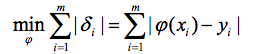
1.使偏差绝对值之和最小
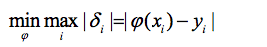
2.使偏差绝对值最大的最小
3.使偏差平方和最小
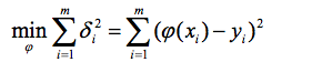
按偏差平方和最小的原则选取拟合曲线,并且采取二项式方程为拟合曲线的方法,称为最小二乘法。
推导过程:
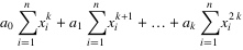
1. 设拟合多项式为:

2. 各点到这条曲线的距离之和,即偏差平方和如下:
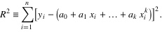
3. 为了求得符合条件的a值,对等式右边求ai偏导数,因而我们得到了:

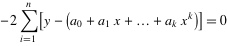
.......
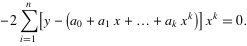
4. 将等式左边进行一下化简,然后应该可以得到下面的等式:
.......
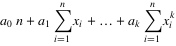
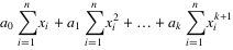
5. 把这些等式表示成矩阵的形式,就可以得到下面的矩阵:
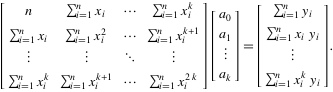
6. 将这个范德蒙得矩阵化简后可得到:
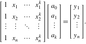
7. 也就是说X*A=Y,那么EA = X'*Y,便得到了系数矩阵A,同时,我们也就得到了拟合曲线。
实现
Matplotlib.pyplot图形库,可用于快速绘制2D图表,与matlab中的plot命令类似,而且用法也基本相同。
plain copy
# coding=utf-8
'''''
作者:Jairus Chan
程序:多项式曲线拟合算法
'''
import matplotlib.pyplot as plt
import math
import numpy
import random
fig = plt.figure()
ax = fig.add_subplot(111)
#阶数为9阶
order=9
#生成曲线上的各个点
x = numpy.arange(-1,1,0.02)
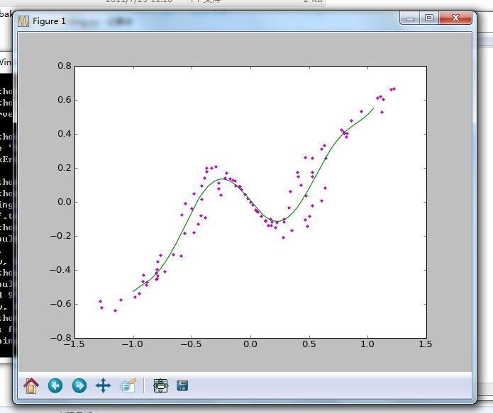
y = [((a*a-1)*(a*a-1)*(a*a-1)+0.5)*numpy.sin(a*2) for a in x]
#ax.plot(x,y,color='r',linestyle='-',marker='')
#,label="(a*a-1)*(a*a-1)*(a*a-1)+0.5"
#生成的曲线上的各个点偏移一下,并放入到xa,ya中去
i=0
xa=[]
ya=[]
for xx in x:
yy=y[i]
d=float(random.randint(60,140))/100
#ax.plot([xx*d],[yy*d],color='m',linestyle='',marker='.')
i+=1
xa.append(xx*d)
ya.append(yy*d)
'''''for i in range(0,5):
xx=float(random.randint(-100,100))/100
yy=float(random.randint(-60,60))/100
xa.append(xx)
ya.append(yy)'''
ax.plot(xa,ya,color='m',linestyle='',marker='.')
#进行曲线拟合
matA=[]
for i in range(0,order+1):
matA1=[]
for j in range(0,order+1):
tx=0.0
for k in range(0,len(xa)):
dx=1.0
for l in range(0,j+i):
dx=dx*xa[k]
tx+=dx
matA1.append(tx)
matA.append(matA1)
#print(len(xa))
#print(matA[0][0])
matA=numpy.array(matA)
matB=[]
for i in range(0,order+1):
ty=0.0
for k in range(0,len(xa)):
dy=1.0
for l in range(0,i):
dy=dy*xa[k]
ty+=ya[k]*dy
matB.append(ty)
matB=numpy.array(matB)
matAA=numpy.linalg.solve(matA,matB)
#画出拟合后的曲线
#print(matAA)
xxa= numpy.arange(-1,1.06,0.01)
yya=[]
for i in range(0,len(xxa)):
yy=0.0
for j in range(0,order+1):
dy=1.0
for k in range(0,j):
dy*=xxa[i]
dy*=matAA[j]
yy+=dy
yya.append(yy)
ax.plot(xxa,yya,color='g',linestyle='-',marker='')
ax.legend()
plt.show()
本博客中所有的博文都为笔者(Jairus Chan)原创。
如需转载,请标明出处:http://blog.csdn.net/JairusChan。
如果您对本文有任何的意见与建议,请联系笔者(JairusChan)。
----------------------------------------------------------java实现,基于Apache数学工具包-------------------------
也可使用Apache开源库commons math,提供的功能更强大,
http://commons.apache.org/proper/commons-math/userguide/fitting.html
[-]
概念
原理
运行前提
代码
运行效果
概念
最小二乘法多项式曲线拟合,根据给定的m个点,并不要求这条曲线精确地经过这些点,而是曲线y=f(x)的近似曲线y= φ(x)。原理
[原理部分由个人根据互联网上的资料进行总结,希望对大家能有用]给定数据点pi(xi,yi),其中i=1,2,…,m。求近似曲线y= φ(x)。并且使得近似曲线与y=f(x)的偏差最小。近似曲线在点pi处的偏差δi= φ(xi)-y,i=1,2,...,m。
常见的曲线拟合方法:
1.使偏差绝对值之和最小
2.使偏差绝对值最大的最小
3.使偏差平方和最小
按偏差平方和最小的原则选取拟合曲线,并且采取二项式方程为拟合曲线的方法,称为最小二乘法。
推导过程:
1. 设拟合多项式为:
2. 各点到这条曲线的距离之和,即偏差平方和如下:
3. 为了求得符合条件的a值,对等式右边求ai偏导数,因而我们得到了:
.......
4. 将等式左边进行一下化简,然后应该可以得到下面的等式:
.......
5. 把这些等式表示成矩阵的形式,就可以得到下面的矩阵:
6. 将这个范德蒙得矩阵化简后可得到:
7. 也就是说X*A=Y,那么EA = X'*Y,便得到了系数矩阵A,同时,我们也就得到了拟合曲线。
实现
运行前提:
Python运行环境与编辑环境;Matplotlib.pyplot图形库,可用于快速绘制2D图表,与matlab中的plot命令类似,而且用法也基本相同。
代码:
[python] viewplain copy
# coding=utf-8
'''''
作者:Jairus Chan
程序:多项式曲线拟合算法
'''
import matplotlib.pyplot as plt
import math
import numpy
import random
fig = plt.figure()
ax = fig.add_subplot(111)
#阶数为9阶
order=9
#生成曲线上的各个点
x = numpy.arange(-1,1,0.02)
y = [((a*a-1)*(a*a-1)*(a*a-1)+0.5)*numpy.sin(a*2) for a in x]
#ax.plot(x,y,color='r',linestyle='-',marker='')
#,label="(a*a-1)*(a*a-1)*(a*a-1)+0.5"
#生成的曲线上的各个点偏移一下,并放入到xa,ya中去
i=0
xa=[]
ya=[]
for xx in x:
yy=y[i]
d=float(random.randint(60,140))/100
#ax.plot([xx*d],[yy*d],color='m',linestyle='',marker='.')
i+=1
xa.append(xx*d)
ya.append(yy*d)
'''''for i in range(0,5):
xx=float(random.randint(-100,100))/100
yy=float(random.randint(-60,60))/100
xa.append(xx)
ya.append(yy)'''
ax.plot(xa,ya,color='m',linestyle='',marker='.')
#进行曲线拟合
matA=[]
for i in range(0,order+1):
matA1=[]
for j in range(0,order+1):
tx=0.0
for k in range(0,len(xa)):
dx=1.0
for l in range(0,j+i):
dx=dx*xa[k]
tx+=dx
matA1.append(tx)
matA.append(matA1)
#print(len(xa))
#print(matA[0][0])
matA=numpy.array(matA)
matB=[]
for i in range(0,order+1):
ty=0.0
for k in range(0,len(xa)):
dy=1.0
for l in range(0,i):
dy=dy*xa[k]
ty+=ya[k]*dy
matB.append(ty)
matB=numpy.array(matB)
matAA=numpy.linalg.solve(matA,matB)
#画出拟合后的曲线
#print(matAA)
xxa= numpy.arange(-1,1.06,0.01)
yya=[]
for i in range(0,len(xxa)):
yy=0.0
for j in range(0,order+1):
dy=1.0
for k in range(0,j):
dy*=xxa[i]
dy*=matAA[j]
yy+=dy
yya.append(yy)
ax.plot(xxa,yya,color='g',linestyle='-',marker='')
ax.legend()
plt.show()
运行效果:
本博客中所有的博文都为笔者(Jairus Chan)原创。
如需转载,请标明出处:http://blog.csdn.net/JairusChan。
如果您对本文有任何的意见与建议,请联系笔者(JairusChan)。
----------------------------------------------------------java实现,基于Apache数学工具包-------------------------
也可使用Apache开源库commons math,提供的功能更强大,
http://commons.apache.org/proper/commons-math/userguide/fitting.html
package com.fjsh.algorithm.leastSquareMethod.deal;

import org.apache.commons.math3.fitting.PolynomialCurveFitter;
import org.apache.commons.math3.fitting.WeightedObservedPoints;

public class LeastSquareMethodFromApache {
private static void testLeastSquareMethodFromApache() {
final WeightedObservedPoints obs = new WeightedObservedPoints();
obs.add(-3, 4);
obs.add(-2, 2);
//        obs.add(-1, 3);
//        obs.add(0, 0);
//        obs.add(1, -1);
//        obs.add(2, -2);
//        obs.add(3, -5);

// Instantiate a third-degree polynomial fitter.
final PolynomialCurveFitter fitter = PolynomialCurveFitter.create(1);

// Retrieve fitted parameters (coefficients of the polynomial function).
final double[] coeff = fitter.fit(obs.toList());
for (double c : coeff) {
System.out.println(c);
}
}

/**
* 例如当参数是PolynomialCurveFitter.create(1);
* 点(-3, 4) (-2, 2) 此时拟合函数参数为-2,-2,公式为y=-2-2x;验证符合
* @param args
*/
public static void main(String[] args) {
testLeastSquareMethodFromApache();
}
}

相关文章推荐
- 最小二乘法多项式曲线拟合原理与实现
- 最小二乘法多项式曲线拟合原理与实现
- 最小二乘法多项式曲线拟合原理与实现
- 最小二乘法多项式曲线拟合原理与实现
- 最小二乘法多项式曲线拟合原理与实现
- 最小二乘法多项式曲线拟合原理与实现
- 最小二乘法多项式曲线拟合原理与实现
- 最小二乘法多项式曲线拟合原理与实现
- 最小二乘法多项式曲线拟合原理与实现 zz
- 最小二乘法多项式曲线拟合原理与实现
- 最小二乘法多项式曲线拟合原理与实现
- 最小二乘法多项式曲线拟合原理与实现(转)
- 最小二乘法多项式曲线拟合原理与实现
- 最小二乘法曲线拟合原理与实现
- 最小二乘法拟合多项式原理以及c++实现
- 最小二乘法多项式拟合的Java实现
- 最小二乘法 多项式曲线拟合 原理公式理解 Python 实现
- 最小二乘法拟合多项式原理以及c++实现
- 最小二乘法拟合多项式曲线原理
- java语言实现简单单链表链式储存结构。插入删除等操作。(有个地方看不出错误来,已经标注,望指正)