zzu数学 实验七几何变换

zzu数学 实验七几何变换

在如photoshop等的各大图形处理软件中，我们能看到各种图形变换，斜切，对称，翻转等，其妙无穷，我们却对其原理一无所知。其实，并不难，今天我以mathematica为例。做两个简单的示例。

示例1

** Linear Transformation **

Clear[f]; t = Pi/6;
a1 = Cos[t]; b1 = -Sin[t]; a2 = Sin[t]; b2 = Cos[t];
f[{x_, y_}] := {a1*x + b1*y, a2*x + b2*y};
co = {}; curve = {};
Do[AppendTo[co, {{-5, y}, {5, y}}], {y, -5, 5}];
Do[AppendTo[co, {{x, -5}, {x, 5}}], {x, -5, 5}];
curve = Table[{1.5 Sin[4 t], -3 Sin[3 t]*Sin[5 t] + 2}, {t, 0, 2 Pi, Pi/180}];
Do[AppendTo[curve, {5 Sin[2 t], 5 Sin[3 t]*Sin[5 t]}], {t, 0, Pi, Pi/180}];
Show[Graphics[Table[Line[co[[i]]], {i, 1, 22}]], Graphics[Line[curve]],
AspectRatio -> Automatic]
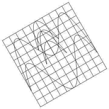
w = 1;
Show[Graphics[
Table[Line[{Nest[f, co[[i, 1]], w], Nest[f, co[[i, 2]], w]}], {i, 1, 22}]],
Graphics[Line[Table[Nest[f, curve[[j]], w], {j, 1, Length[curve]}]]],
AspectRatio -> Automatic]

Clear[f];
a1 = 1.1; b1 = 0.3; a2 = 0.2; b2 = 0.9;
f[{x_, y_}] := {a1*x + b1*y, a2*x + b2*y};
w = 1;
Show[Graphics[
Table[Line[{Nest[f, co[[i, 1]], w], Nest[f, co[[i, 2]], w]}], {i, 1, 22}]],
Graphics[Line[Table[Nest[f, curve[[j]], w], {j, 1, Length[curve]}]]],
AspectRatio -> Automatic]

pic={};n=90;
Do[p0={Cos[2m*Pi/n],Sin[2m*Pi/n]};
AppendTo[pic,Line[{{0,0},2p0}]];
points={};p=p0;Do[AppendTo[points,p];p1=f[p];p=p1,{k,1,2}];
AppendTo[pic,Line[points]],
{m,1,n}];
pic1=Show[Graphics[pic],AspectRatio->Automatic]

co = {}; curve = {};
Do[AppendTo[
co, {{-5 - 0.8229 y, -5*0.5486 + y}, {5 - 0.8229 y,
5*0.5486 + y}}], {y, -5, 5}];
Do[AppendTo[
co, {{x + 5*0.8229, 0.5486 x - 5}, {x - 5*0.8229, 0.5486 x + 5}}], {x, -5,
5}];
curve = Table[{1.5 Sin[4 t], -3 Sin[3 t]*Sin[5 t] + 2}, {t, 0, 2 Pi, Pi/180}];
Do[AppendTo[curve, {5 Sin[2 t], 5 Sin[3 t]*Sin[5 t]}], {t, 0, Pi, Pi/180}];
Show[Graphics[Table[Line[co[[i]]], {i, 1, 22}]], Graphics[Line[curve]],
AspectRatio -> Automatic]
w = 1;
Show[Graphics[
Table[Line[{Nest[f, co[[i, 1]], w], Nest[f, co[[i, 2]], w]}], {i, 1, 22}]],
Graphics[Line[Table[Nest[f, curve[[j]], w], {j, 1, Length[curve]}]]],
AspectRatio -> Automatic]

pic={};
Do[x=2Random[]-1;y=2Random[]-1;s={x,y};
Do[AppendTo[pic,s];s1=f[s];s=s1
,{h,1,7}]
,{m,1,200}];
ListPlot[pic,AspectRatio->Automatic]

A = {{1, 0.5, 0.4}, {2, 1, 0.7}, {2.5, 1.0/0.7, 2}}; B = {1, 1, 1};
Do[B1 = A.B; c = Apply[Plus, B1]; B2 = B1/c; Print[B2]; B = B2,
{n, 1, 9}]

b = 0.5;  Clear[t];
g[{x_, y_}] := {x/(1 - x), y/(1 - x)};
line1 = {t + 1, 0.1 t + b}; line2 = {t + 1,
t + b}; line3 = {t + 1, -0.5 t + b}; line4 = {t + 1, -1.5 t + b};
ParametricPlot[{line1, line2, line3, line4}, {t, -1, 1.5},
AspectRatio -> Automatic];
ParametricPlot[{g[line1], g[line2], g[line3], g[line4]}, {t, -10, 10},
AspectRatio -> Automatic]

u = ArcCos[1/1.3];
p1 = {0.8 Cos[t], 0.8 Sin[t]}; p2 = {1.0 Cos[t],
1.0 Sin[t]}; p3 = {1.3 Cos[t*u/Pi - u], 1.3 Sin[t*u/Pi - u]};
p4 = {1.3 Cos[t*(Pi - u)/Pi + u], 1.3 Sin[t*(Pi - u)/Pi + u]};
ParametricPlot[{p1, p2, p3, p4}, {t, 0, 2 Pi}, AspectRatio -> Automatic];
ParametricPlot[{g[p1], g[p2], g[p3], g[p4]}, {t, 0, 2 Pi},
AspectRatio -> Automatic]

p4={2Cos[t],2Sin[t]};
pic41=ParametricPlot[p4,{t,-Pi/3,Pi/3},PlotStyle->{RGBColor[1,0,0]},AspectRatio->Automatic->True];
pic42=ParametricPlot[p4,{t,Pi/3,5Pi/3},PlotStyle->{RGBColor[0,0,1]},AspectRatio->Automatic->True];
Show[pic41,pic42]

pic51=ParametricPlot[g[p4],{t,-Pi/3,Pi/3},PlotStyle->{RGBColor[1,0,0]},AspectRatio->Automatic->True];
pic52=ParametricPlot[g[p4],{t,Pi/3,5Pi/3},PlotStyle->{RGBColor[0,0,1]},AspectRatio->Automatic->True];
Show[pic51,pic52]

Clear[f];
t=0.05;
f[{x_,y_}]:={(x*Cosh[t]+Sinh[t])/(x*Sinh[t]+Cosh[t]),y/(x*Sinh[t]+Cosh[t])};
pic1=ParametricPlot[{Cos[u],Sin[u]},{u,0,2Pi},PlotStyle->{RGBColor[1,0,0]},AspectRatio->Automatic];
p={0,0};ta={};
Do[AppendTo[ta,Line[{p,{p[[1]],0.1}}]];AppendTo[ta,Line[{-p,{-p[[1]],0.1}}]];
p1=f[p];p=p1, {n,1,30}];
Show[pic1,Graphics[ta]]

Clear[f]; t = 1.0;
f[{x_, y_}] := {(x*Cosh[t] + Sinh[t])/(x*Sinh[t] + Cosh[t]),
y/(x*Sinh[t] + Cosh[t])};
tb = Table[Line[{f[{0, 0}], f[{Cos[k], Sin[k]}]}], {k, 0, 2 Pi, Pi/12}];
Show[pic1, Graphics[tb]]

Show[pic1,
Graphics[{Line[{{-1, 0}, {Cos[1], Sin[1]}}],
Line[{{1, 0}, {Cos[2.5], Sin[2.5]}}]}]]

** Roots of complex polynormials **

f[z_] := z^4 - (3 + 4 I)*z^2 + 2.5 z - 10 ;
g[{r_, t_}] := {Re[f[r (Cos[t] + Sin[t]*I)]], Im[f[r (Cos[t] + Sin[t]*I)]]};
r = 5.487;
ParametricPlot[g[{r, t}], {t, 0, 2 Pi}, AspectRatio -> Automatic]

rsquare[t_] := Apply[Plus, g[{r, t}]^2];
Plot[rsquare[t], {t, 0.362218, 0.361987}]

FindMinimum[rsquare[t], {t, 0.36}]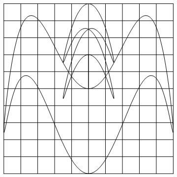

- 示例2

n = 100; ratio = 1.5;
pi0 = Table[{Cos[2*k*Pi/n], Sin[2*k*Pi/n]}, {k, 0, n - 1}];
pi1 = ratio*pi0;
a = Graphics[{Red, Line[Table[{{0, 0}, pi1[[i]]}, {i, 1, n}]]}];
A = {{1, 0.5}, {0.5, 1}};
pi2 = Table[A.pi0[[i]], {i, 1, n}];
b = Graphics[Line[Table[{pi0[[i]], pi2[[i]]}, {i, 1, n}]]];
Show[a, b]

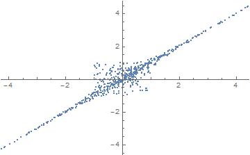
n = 100; k = 5;
pi = RandomReal[{-1, 1}, {n, 2}];
pointgroup = {pi};
A = {{1, 0.5}, {0.5, 1}};
For[i = 1, i <= k, i++, pi = pi.A;
AppendTo[pointgroup, pi]];
pointgroup = Flatten[pointgroup, 1];
ListPlot[pointgroup]

A={1,1.1}
B=Eigenvectors[m]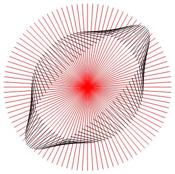

图比较多，我就不一一贴上来了，大家运行一下就可以看到效果。有什么需要讨论的，可以私信给我。