简单线性回归
2016-09-08 15:51
218 查看
协方差:两个变量总体误差的期望。
简单的说就是度量Y和X之间关系的方向和强度。
X :预测变量
Y :响应变量
View Code
================================
校验假设:
虽然上面的实例算出了线性关系,但是我们怎么判断我们开始预设立得假设呢,就是我们是否要推翻假设,毕竟是假设,
假设未来一周我有一个亿,根据现实偏离太大,估计会推翻假设。
算了还是切入正题吧:
开始我假设了个模型:

我们需要校验这个假设,我们还要附加假定:
对于X的每一个固定值,所以的ε都相互独立,并且都服从均值为0,方程为σ方 的正态分布


得到:

SSE为残差,n-2为自由度[自由度=观测个数-待估回归参数个数]
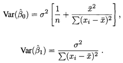
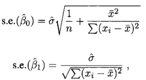
带入化简得倒,标准误差分别是:


的标准误差刻画了斜率的估计精度,标准误越小估计精度越高
简单的说就是度量Y和X之间关系的方向和强度。
X :预测变量
Y :响应变量
def lsqr(A, b, damp=0.0, atol=1e-8, btol=1e-8, conlim=1e8,
iter_lim=None, show=False, calc_var=False):
"""Find the least-squares solution to a large, sparse, linear system
of equations.

The function solves ``Ax = b``  or  ``min ||b - Ax||^2`` or
``min ||Ax - b||^2 + d^2 ||x||^2``.

The matrix A may be square or rectangular (over-determined or
under-determined), and may have any rank.

::

1. Unsymmetric equations --    solve  A*x = b

2. Linear least squares  --    solve  A*x = b
in the least-squares sense

3. Damped least squares  --    solve  (   A    )*x = ( b )
( damp*I )     ( 0 )
in the least-squares sense

Parameters
----------
A : {sparse matrix, ndarray, LinearOperatorLinear}
Representation of an m-by-n matrix.  It is required that
the linear operator can produce ``Ax`` and ``A^T x``.
b : (m,) ndarray
Right-hand side vector ``b``.
damp : float
Damping coefficient.
atol, btol : float
Stopping tolerances. If both are 1.0e-9 (say), the final
residual norm should be accurate to about 9 digits.  (The
final x will usually have fewer correct digits, depending on
cond(A) and the size of damp.)
conlim : float
Another stopping tolerance.  lsqr terminates if an estimate of
``cond(A)`` exceeds `conlim`.  For compatible systems ``Ax =
b``, `conlim` could be as large as 1.0e+12 (say).  For
least-squares problems, conlim should be less than 1.0e+8.
Maximum precision can be obtained by setting ``atol = btol =
conlim = zero``, but the number of iterations may then be
excessive.
iter_lim : int
Explicit limitation on number of iterations (for safety).
show : bool
Display an iteration log.
calc_var : bool
Whether to estimate diagonals of ``(A'A + damp^2*I)^{-1}``.

Returns
-------
x : ndarray of float
The final solution.
istop : int
Gives the reason for termination.
1 means x is an approximate solution to Ax = b.
2 means x approximately solves the least-squares problem.
itn : int
Iteration number upon termination.
r1norm : float
``norm(r)``, where ``r = b - Ax``.
r2norm : float
``sqrt( norm(r)^2  +  damp^2 * norm(x)^2 )``.  Equal to `r1norm` if
``damp == 0``.
anorm : float
Estimate of Frobenius norm of ``Abar = [[A]; [damp*I]]``.
acond : float
Estimate of ``cond(Abar)``.
arnorm : float
Estimate of ``norm(A'*r - damp^2*x)``.
xnorm : float
``norm(x)``
var : ndarray of float
If ``calc_var`` is True, estimates all diagonals of
``(A'A)^{-1}`` (if ``damp == 0``) or more generally ``(A'A +
damp^2*I)^{-1}``.  This is well defined if A has full column
rank or ``damp > 0``.  (Not sure what var means if ``rank(A)
< n`` and ``damp = 0.``)

Notes
-----
LSQR uses an iterative method to approximate the solution.  The
number of iterations required to reach a certain accuracy depends
strongly on the scaling of the problem.  Poor scaling of the rows
or columns of A should therefore be avoided where possible.

For example, in problem 1 the solution is unaltered by
row-scaling.  If a row of A is very small or large compared to
the other rows of A, the corresponding row of ( A  b ) should be
scaled up or down.

In problems 1 and 2, the solution x is easily recovered
following column-scaling.  Unless better information is known,
the nonzero columns of A should be scaled so that they all have
the same Euclidean norm (e.g., 1.0).

In problem 3, there is no freedom to re-scale if damp is
nonzero.  However, the value of damp should be assigned only
after attention has been paid to the scaling of A.

The parameter damp is intended to help regularize
ill-conditioned systems, by preventing the true solution from
being very large.  Another aid to regularization is provided by
the parameter acond, which may be used to terminate iterations
before the computed solution becomes very large.

If some initial estimate ``x0`` is known and if ``damp == 0``,
one could proceed as follows:

1. Compute a residual vector ``r0 = b - A*x0``.
2. Use LSQR to solve the system  ``A*dx = r0``.
3. Add the correction dx to obtain a final solution ``x = x0 + dx``.

This requires that ``x0`` be available before and after the call
to LSQR.  To judge the benefits, suppose LSQR takes k1 iterations
to solve A*x = b and k2 iterations to solve A*dx = r0.
If x0 is "good", norm(r0) will be smaller than norm(b).
If the same stopping tolerances atol and btol are used for each
system, k1 and k2 will be similar, but the final solution x0 + dx
should be more accurate.  The only way to reduce the total work
is to use a larger stopping tolerance for the second system.
If some value btol is suitable for A*x = b, the larger value
btol*norm(b)/norm(r0)  should be suitable for A*dx = r0.

Preconditioning is another way to reduce the number of iterations.
If it is possible to solve a related system ``M*x = b``
efficiently, where M approximates A in some helpful way (e.g. M -
A has low rank or its elements are small relative to those of A),
LSQR may converge more rapidly on the system ``A*M(inverse)*z =
b``, after which x can be recovered by solving M*x = z.

If A is symmetric, LSQR should not be used!

Alternatives are the symmetric conjugate-gradient method (cg)
and/or SYMMLQ.  SYMMLQ is an implementation of symmetric cg that
applies to any symmetric A and will converge more rapidly than
LSQR.  If A is positive definite, there are other implementations
of symmetric cg that require slightly less work per iteration than
SYMMLQ (but will take the same number of iterations).

References
----------
.. [1] C. C. Paige and M. A. Saunders (1982a).
"LSQR: An algorithm for sparse linear equations and
sparse least squares", ACM TOMS 8(1), 43-71.
.. [2] C. C. Paige and M. A. Saunders (1982b).
"Algorithm 583.  LSQR: Sparse linear equations and least
squares problems", ACM TOMS 8(2), 195-209.
.. [3] M. A. Saunders (1995).  "Solution of sparse rectangular
systems using LSQR and CRAIG", BIT 35, 588-604.

"""
A = aslinearoperator(A)
if len(b.shape) > 1:
b = b.squeeze()

m, n = A.shape
if iter_lim is None:
iter_lim = 2 * n
var = np.zeros(n)

msg = ('The exact solution is  x = 0                              ',
'Ax - b is small enough, given atol, btol                  ',
'The least-squares solution is good enough, given atol     ',
'The estimate of cond(Abar) has exceeded conlim            ',
'Ax - b is small enough for this machine                   ',
'The least-squares solution is good enough for this machine',
'Cond(Abar) seems to be too large for this machine         ',
'The iteration limit has been reached                      ')

itn = 0
istop = 0
nstop = 0
ctol = 0
if conlim > 0:
ctol = 1/conlim
anorm = 0
acond = 0
dampsq = damp**2
ddnorm = 0
res2 = 0
xnorm = 0
xxnorm = 0
z = 0
cs2 = -1
sn2 = 0

"""
Set up the first vectors u and v for the bidiagonalization.
These satisfy  beta*u = b,  alfa*v = A'u.
"""
__xm = np.zeros(m)  # a matrix for temporary holding
__xn = np.zeros(n)  # a matrix for temporary holding
v = np.zeros(n)
u = b
x = np.zeros(n)
alfa = 0
beta = np.linalg.norm(u)
w = np.zeros(n)

if beta > 0:
u = (1/beta) * u
v = A.rmatvec(u)
alfa = np.linalg.norm(v)

if alfa > 0:
v = (1/alfa) * v
w = v.copy()

rhobar = alfa
phibar = beta
bnorm = beta
rnorm = beta
r1norm = rnorm
r2norm = rnorm

# Reverse the order here from the original matlab code because
# there was an error on return when arnorm==0
arnorm = alfa * beta
if arnorm == 0:
print(msg[0])
return x, istop, itn, r1norm, r2norm, anorm, acond, arnorm, xnorm, var

head1 = '   Itn      x[0]       r1norm     r2norm '
head2 = ' Compatible    LS      Norm A   Cond A'

if show:
print(' ')
print(head1, head2)
test1 = 1
test2 = alfa / beta
str1 = '%6g %12.5e' % (itn, x[0])
str2 = ' %10.3e %10.3e' % (r1norm, r2norm)
str3 = '  %8.1e %8.1e' % (test1, test2)
print(str1, str2, str3)

# Main iteration loop.
while itn < iter_lim:
itn = itn + 1
"""
%     Perform the next step of the bidiagonalization to obtain the
%     next  beta, u, alfa, v.  These satisfy the relations
%                beta*u  =  a*v   -  alfa*u,
%                alfa*v  =  A'*u  -  beta*v.
"""
u = A.matvec(v) - alfa * u
beta = np.linalg.norm(u)

if beta > 0:
u = (1/beta) * u
anorm = sqrt(anorm**2 + alfa**2 + beta**2 + damp**2)
v = A.rmatvec(u) - beta * v
alfa = np.linalg.norm(v)
if alfa > 0:
v = (1 / alfa) * v

# Use a plane rotation to eliminate the damping parameter.
# This alters the diagonal (rhobar) of the lower-bidiagonal matrix.
rhobar1 = sqrt(rhobar**2 + damp**2)
cs1 = rhobar / rhobar1
sn1 = damp / rhobar1
psi = sn1 * phibar
phibar = cs1 * phibar

# Use a plane rotation to eliminate the subdiagonal element (beta)
# of the lower-bidiagonal matrix, giving an upper-bidiagonal matrix.
cs, sn, rho = _sym_ortho(rhobar1, beta)

theta = sn * alfa
rhobar = -cs * alfa
phi = cs * phibar
phibar = sn * phibar
tau = sn * phi

# Update x and w.
t1 = phi / rho
t2 = -theta / rho
dk = (1 / rho) * w

x = x + t1 * w
w = v + t2 * w
ddnorm = ddnorm + np.linalg.norm(dk)**2

if calc_var:
var = var + dk**2

# Use a plane rotation on the right to eliminate the
# super-diagonal element (theta) of the upper-bidiagonal matrix.
# Then use the result to estimate norm(x).
delta = sn2 * rho
gambar = -cs2 * rho
rhs = phi - delta * z
zbar = rhs / gambar
xnorm = sqrt(xxnorm + zbar**2)
gamma = sqrt(gambar**2 + theta**2)
cs2 = gambar / gamma
sn2 = theta / gamma
z = rhs / gamma
xxnorm = xxnorm + z**2

# Test for convergence.
# First, estimate the condition of the matrix  Abar,
# and the norms of  rbar  and  Abar'rbar.
acond = anorm * sqrt(ddnorm)
res1 = phibar**2
res2 = res2 + psi**2
rnorm = sqrt(res1 + res2)
arnorm = alfa * abs(tau)

# Distinguish between
#    r1norm = ||b - Ax|| and
#    r2norm = rnorm in current code
#           = sqrt(r1norm^2 + damp^2*||x||^2).
#    Estimate r1norm from
#    r1norm = sqrt(r2norm^2 - damp^2*||x||^2).
# Although there is cancellation, it might be accurate enough.
r1sq = rnorm**2 - dampsq * xxnorm
r1norm = sqrt(abs(r1sq))
if r1sq < 0:
r1norm = -r1norm
r2norm = rnorm

# Now use these norms to estimate certain other quantities,
# some of which will be small near a solution.
test1 = rnorm / bnorm
test2 = arnorm / (anorm * rnorm)
test3 = 1 / acond
t1 = test1 / (1 + anorm * xnorm / bnorm)
rtol = btol + atol * anorm * xnorm / bnorm

# The following tests guard against extremely small values of
# atol, btol  or  ctol.  (The user may have set any or all of
# the parameters  atol, btol, conlim  to 0.)
# The effect is equivalent to the normal tests using
# atol = eps,  btol = eps,  conlim = 1/eps.
if itn >= iter_lim:
istop = 7
if 1 + test3 <= 1:
istop = 6
if 1 + test2 <= 1:
istop = 5
if 1 + t1 <= 1:
istop = 4

# Allow for tolerances set by the user.
if test3 <= ctol:
istop = 3
if test2 <= atol:
istop = 2
if test1 <= rtol:
istop = 1

# See if it is time to print something.
prnt = False
if n <= 40:
prnt = True
if itn <= 10:
prnt = True
if itn >= iter_lim-10:
prnt = True
# if itn%10 == 0: prnt = True
if test3 <= 2*ctol:
prnt = True
if test2 <= 10*atol:
prnt = True
if test1 <= 10*rtol:
prnt = True
if istop != 0:
prnt = True

if prnt:
if show:
str1 = '%6g %12.5e' % (itn, x[0])
str2 = ' %10.3e %10.3e' % (r1norm, r2norm)
str3 = '  %8.1e %8.1e' % (test1, test2)
str4 = ' %8.1e %8.1e' % (anorm, acond)
print(str1, str2, str3, str4)

if istop != 0:
break

# End of iteration loop.

return x, istop, itn, r1norm, r2norm, anorm, acond, arnorm, xnorm, var
View Code
================================
校验假设:
虽然上面的实例算出了线性关系,但是我们怎么判断我们开始预设立得假设呢,就是我们是否要推翻假设,毕竟是假设,
假设未来一周我有一个亿,根据现实偏离太大,估计会推翻假设。
算了还是切入正题吧:
开始我假设了个模型:

我们需要校验这个假设,我们还要附加假定:
对于X的每一个固定值,所以的ε都相互独立,并且都服从均值为0,方程为σ方 的正态分布


得到:

SSE为残差,n-2为自由度[自由度=观测个数-待估回归参数个数]
带入化简得倒,标准误差分别是:


的标准误差刻画了斜率的估计精度,标准误越小估计精度越高
相关文章推荐
- 7.1简单线性回归--python机器学习
- R语言简单(一元)线性回归分析
- 简单线性回归
- pytho简单线性回归
- Python3 安装 numpy 科学库 简单线性回归
- 简单线性回归分析【笔记】
- 基于tensorflow的简单线性回归实例
- 简单线性回归
- R语言写简单线性回归
- 用PHP实现的简单线性回归
- PHP实现简单线性回归之数据研究工具(1)
- 简单线性回归的随机梯度下降算法实现:Linear Regression - SGD
- 简单线性回归
- 简单线性回归的Python实现
- tensorflow入门Day1-简单线性回归
- 使用Eviews做简单线性回归
- 多元线性回归、梯度下降法、正规方程法简单实验
- R语言基础入门之五:简单线性回归
- 机器学习练习(一)——简单线性回归
- 运用TensorFlow进行简单实现线性回归、梯度下降示例
