Convolutional neural networks(CNN) (三) Sparse Autoencoder Exercise(Vectorization)
2016-07-30 11:28
477 查看
{作为CNN学习入门的一部分,笔者在这里逐步给出UFLDL的各章节Exercise的个人代码实现,供大家参考指正}
此文紧承上篇Blog,是对Sparse
Autoencoder Exercise的向量化优化,按照要求只修改了SparseAutoEncoderCost.m。
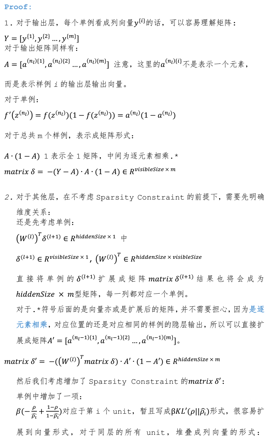
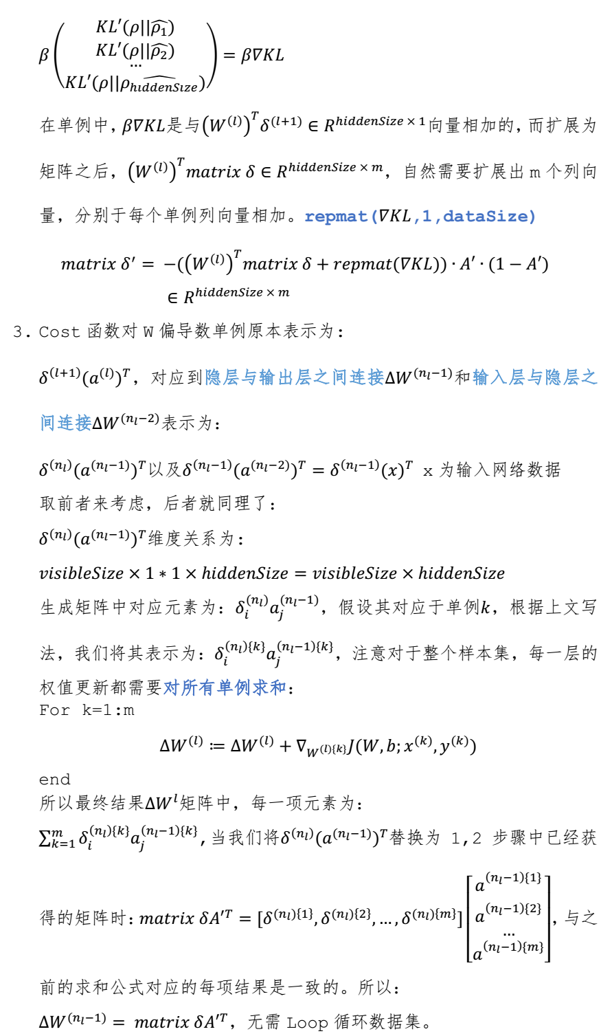
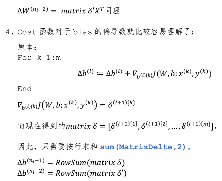
将所有的Loop操作以向量化的方式优化实现,下面先给出证明,比较冗长,适用于之前对向量化表示不是很熟悉的读者:

下面给出原方法与Vectorization后的速度比较,由于笔者对函数也进行了删减,已达到更快的速度,所以前后版本部分函数不一致:
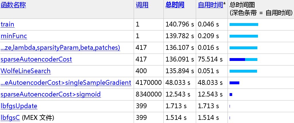
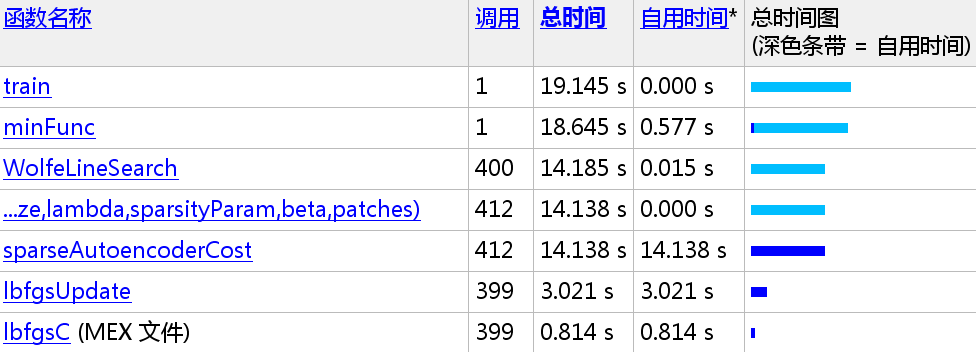
136.091/14.138 =
9.6259x
笔者的计算环境为i7-5500U + 16G内存 MatLab 2014a
下面给出sparseAutoEncoderCost.m:

此文紧承上篇Blog,是对Sparse
Autoencoder Exercise的向量化优化,按照要求只修改了SparseAutoEncoderCost.m。
将所有的Loop操作以向量化的方式优化实现,下面先给出证明,比较冗长,适用于之前对向量化表示不是很熟悉的读者:
下面给出原方法与Vectorization后的速度比较,由于笔者对函数也进行了删减,已达到更快的速度,所以前后版本部分函数不一致:
136.091/14.138 =
9.6259x
笔者的计算环境为i7-5500U + 16G内存 MatLab 2014a
下面给出sparseAutoEncoderCost.m:
function [cost,grad] = sparseAutoencoderCost(theta, visibleSize, hiddenSize, ...
lambda, sparsityParam, beta, data)

% visibleSize: the number of input units (probably 64)
% hiddenSize: the number of hidden units (probably 25)
% lambda: weight decay parameter
% sparsityParam: The desired average activation for the hidden units (denoted in the lecture
%                           notes by the greek alphabet rho, which looks like a lower-case "p").
% beta: weight of sparsity penalty term
% data: Our 64x10000 matrix containing the training data.  So, data(:,i) is the i-th training example.

% The input theta is a vector (because minFunc expects the parameters to be a vector).
% We first convert theta to the (W1, W2, b1, b2) matrix/vector format, so that this
% follows the notation convention of the lecture notes.

W1 = reshape(theta(1:hiddenSize*visibleSize), hiddenSize, visibleSize);
W2 = reshape(theta(hiddenSize*visibleSize+1:2*hiddenSize*visibleSize), visibleSize, hiddenSize);
b1 = theta(2*hiddenSize*visibleSize+1:2*hiddenSize*visibleSize+hiddenSize);
b2 = theta(2*hiddenSize*visibleSize+hiddenSize+1:end);

% Cost and gradient variables (your code needs to compute these values).
% Here, we initialize them to zeros.
% cost = 0; No need to initialize cost.
% W1grad = zeros(size(W1));
% W2grad = zeros(size(W2));
% b1grad = zeros(size(b1));
% b2grad = zeros(size(b2));

%% ---------- YOUR CODE HERE --------------------------------------
%  Instructions: Compute the cost/optimization objective J_sparse(W,b) for the Sparse Autoencoder,
%                and the corresponding gradients W1grad, W2grad, b1grad, b2grad.
%
% W1grad, W2grad, b1grad and b2grad should be computed using backpropagation.
% Note that W1grad has the same dimensions as W1, b1grad has the same dimensions
% as b1, etc.  Your code should set W1grad to be the partial derivative of J_sparse(W,b) with
% respect to W1.  I.e., W1grad(i,j) should be the partial derivative of J_sparse(W,b)
% with respect to the input parameter W1(i,j).  Thus, W1grad should be equal to the term
% [(1/m) \Delta W^{(1)} + \lambda W^{(1)}] in the last block of pseudo-code in Section 2.2
% of the lecture notes (and similarly for W2grad, b1grad, b2grad).
%
% Stated differently, if we were using batch gradient descent to optimize the parameters,
% the gradient descent update to W1 would be W1 := W1 - alpha * W1grad, and similarly for W2, b1, b2.
%

dataSize = 10000;
% WARNING !! Original value = 10000. You may change it to test your gradient calculation result.
% dataSize = 10;

% J_w_b_Vec = zeros(dataSize,1);
% ActivationMatrix2 = zeros(hiddenSize, dataSize); % activation equals output
% ActivationMatrix3 = zeros(visibleSize, dataSize); % activation equals output

% DelteW1 = zeros(size(W1));
% DelteW2 = zeros(size(W2));
% Delteb1 = zeros(size(b1));
% Delteb2 = zeros(size(b2));

% define loss function:
% (1/2) * || y - H_w_b(x) || ^2 + Regularization term + Sparsity Constraint
MatrixZ2 = W1 * data + repmat(b1,1,dataSize);
MatrixA2 = 1 ./ (1 + exp(-MatrixZ2));
MatrixZ3 = W2 * MatrixA2 + repmat(b2,1,dataSize);
MatrixA3 = 1 ./ (1 + exp(-MatrixZ3));
MatrixDiff = MatrixA3 - data;
J_w_b_Vec = sum(MatrixDiff.^2)./2;

% for i = 1:1:dataSize
%     z2 = W1 * data(:,i) + b1;
%     a2 = sigmoid(z2);
%     ActivationMatrix2(:,i) = a2;
%     z3 = W2 * a2 + b2;
%     a3 = sigmoid(z3);
%     ActivationMatrix3(:,i) = a3;
%     diff = a3 - data(:,i);
%     J_w_b_Vec(i) = sum((diff.^2))/2;
% end

% Regularizatio
d8d9
n term
WeightDecay = lambda/2 * (sum(sum(W1.^2)) + sum(sum(W2.^2)));
% Sparsity Constraint term
pVec = sum(MatrixA2,2)/dataSize; % row sum
KL = beta * sum(sparsityParam*(log(sparsityParam) - log(pVec)) ...
+ (1-sparsityParam)*(log(1-sparsityParam)-log(1-pVec)));

cost = sum(J_w_b_Vec)/dataSize + WeightDecay + KL;

MatrixDelte_nl = -(data - MatrixA3).*(MatrixA3.*(1 - MatrixA3));
% size(W2)
% size(MatrixDelte_nl)
% size(repmat(pVec,1,visibleSize))
% size(MatrixA2)

MatrixDelte_hidden = ((W2)'*MatrixDelte_nl + ...
beta*(-sparsityParam./repmat(pVec,1,dataSize) + ...
(1-sparsityParam)./(1-repmat(pVec,1,dataSize)))).* ...
(MatrixA2.*(1 - MatrixA2));

% Compute the desired partial derivatives per layer
% Output Layer : nl
MatrixWLgradient_nl = MatrixDelte_nl * (MatrixA2)';
MatrixbLgradient_nl = sum(MatrixDelte_nl,2);
% Hidden Layer : nl - 1
MatrixWLgradient_hidden = MatrixDelte_hidden * (data)';
MatrixbLgradient_hidden = sum(MatrixDelte_hidden,2);

% size(MatrixWLgradient_nl)
% size(MatrixbLgradient_nl)
% size(MatrixWLgradient_hidden)
% size(MatrixbLgradient_hidden)

% for i = 1:1:dataSize
%     [dW1, db1, dW2, db2] = singleSampleGradient(data(:,i), ...
%                                                 ActivationMatrix2(:,i), ...
%                                                 ActivationMatrix3(:,i), ...
%                                                 W2, ...
%                                                 beta, ...
%                                                 pVec, ...
%                                                 sparsityParam);
%     DelteW1 = DelteW1 + dW1;
%     DelteW2 = DelteW2 + dW2;
%     Delteb1 = Delteb1 + db1;
%     Delteb2 = Delteb2 + db2;
%
% end

W1grad = MatrixWLgradient_hidden / dataSize + lambda * W1;
W2grad = MatrixWLgradient_nl / dataSize + lambda * W2;
b1grad = MatrixbLgradient_hidden / dataSize;
b2grad = MatrixbLgradient_nl / dataSize;

%-------------------------------------------------------------------
% After computing the cost and gradient, we will convert the gradients back
% to a vector format (suitable for minFunc).  Specifically, we will unroll
% your gradient matrices into a vector.

grad = [W1grad(:) ; W2grad(:) ; b1grad(:) ; b2grad(:)];

end

%-------------------------------------------------------------------
% Here's an implementation of the sigmoid function, which you may find useful
% in your computation of the costs and the gradients.  This inputs a (row or
% column) vector (say (z1, z2, z3)) and returns (f(z1), f(z2), f(z3)).

% Single Sample
% function [WLgradient_hidden, bLgradient_hidden, WLgradient_nl, bLgradient_nl] = ...
%     singleSampleGradient(data, ActivationVec_hidden, ActivationVec_nl, W2, beta, pVec, sparsityParam)
%
% % Delte_nl = zeros(size(ActivationVec_nl));
% % Delte_hidden = zeros(size(ActivationVec_hidden));
%
% % Compute error terms per layer
% % Output Layer : nl
% Delte_nl = -(data - ActivationVec_nl).*(ActivationVec_nl.*(1 - ActivationVec_nl));
% % Hidden Layer : nl - 1 without sparsity constraint
% % Delte_hidden = ((W2)'*Delte_nl).*(ActivationVec_hidden.*(1 - ActivationVec_hidden));
% % Hidden Layer : nl - 1 with sparsity constraint
% Delte_hidden = ((W2)'*Delte_nl + beta*(-sparsityParam./pVec + (1-sparsityParam)./(1-pVec))).* ...
%     (ActivationVec_hidden.*(1 - ActivationVec_hidden));
%
% % Compute the desired partial derivatives per layer
% % Output Layer : nl
% WLgradient_nl = Delte_nl * (ActivationVec_hidden)';
% bLgradient_nl = Delte_nl;
% % Hidden Layer : nl - 1
% WLgradient_hidden = Delte_hidden * (data)';
% bLgradient_hidden = Delte_hidden;
%
% end
实验结果:

相关文章推荐
- CUDA搭建
- 深入理解CNN的细节
- TensorFlow人工智能引擎入门教程所有目录
- convolutional neural network
- UFLDL Exercise: Convolutional Neural Network
- 使用深度卷积网络和支撑向量机实现的商标检测与分类的例子
- 对Pedestrian Detection aided by Deep Learning Semantic Tasks的小结
- CNN学习(一)
- CNN学习(一)
- UFLDL稀疏编码器练习实现
- UFLDL矢量化编程练习:翻译
- UFLDL矢量化编程练习:遇到问题
- UFLDL矢量化编程练习:用MNIST数据集的稀疏自编码器训练实现
- 阅读 理解 思考 - Learning to Segment Object Candidates
- 卷积神经网络学习
- CNN: single-label to multi-label总结
- 总结:Large Scale Distributed Deep Networks
- 总结:One weird trick for parallelizing convolutional neural networks
- Sparse Autoencoder 编程练习