Triplet Loss、Coupled Cluster Loss 探究

Preface

因为要区分相似图像，所以研究了一下 Triplet Loss，还有今年 CVPR 的一篇文章：《Deep Relative Distance Learning: Tell the Difference Between Similar Vehicles》，这篇文章提出了 Coupled Cluster Loss 。

文章的主要内容在之前的阅读笔记已经叙述过了，文本主要集中于对这两个损失函数的实验部分。

Triplet Loss

Triplet Loss 的 Torch 实验

Triplet Loss 的 Torch 实现，有人已经做好了。只需看懂即可，看看是怎么做的。为接下去实现 Coupled Cluster Loss 做好准备。

具体参见这里的 Github 仓库，Google 的《FaceNet: A Unified Embedding for Face Recognition and Clustering 》 论文就是用的这个 Triplet Loss 实现 ，代码参见：https://github.com/cmusatyalab/openface

贴上主要实现部分：

--------------------------------------------------------------------------------
-- TripletEmbeddingCriterion
--------------------------------------------------------------------------------
-- Alfredo Canziani, Apr/May 15
-- Xinpeng.Chen --
--------------------------------------------------------------------------------

local TripletEmbeddingCriterion, parent = torch.class('nn.TripletEmbeddingCriterion', 'nn.Criterion')

function TripletEmbeddingCriterion:__init(alpha)
parent.__init(self)
self.alpha = alpha or 0.2
self.Li = torch.Tensor()
self.gradInput = {}
end

function TripletEmbeddingCriterion:updateOutput(input)
local a = input[1] -- anchor
local p = input[2] -- positive
local n = input[3] -- negative
local N = a:size(1) -- N is batchSize, represent the N in the formula
self.Li:resize(N)
for i = 1, N do
self.Li[i] = math.max(0, (a[i] - p[i]) * (a[i] - p[i]) + self.alpha - (a[i] - n[i]) * (a[i] - n[i]))
end
self.output = self.Li:sum() / N

return self.output
end

function TripletEmbeddingCriterion:updateGradInput(input)
local a = input[1] -- anchor
local p = input[2] -- positive
local n = input[3] -- negative
local N = a:size(1) -- N is batchSize, represent the N in the formula
if torch.type(a) == 'torch.CudaTensor' then -- if buggy CUDA API
self.gradInput[1] = (n - p):cmul(self.Li:gt(0):repeatTensor(a:size(2),1):t():type(a:type()) * 2/N)
self.gradInput[2] = (p - a):cmul(self.Li:gt(0):repeatTensor(a:size(2),1):t():type(a:type()) * 2/N)
self.gradInput[3] = (a - n):cmul(self.Li:gt(0):repeatTensor(a:size(2),1):t():type(a:type()) * 2/N)
else -- otherwise
self.gradInput[1] = self.Li:gt(0):diag():type(a:type()) * (n - p) * 2/N
self.gradInput[2] = self.Li:gt(0):diag():type(a:type()) * (p - a) * 2/N
self.gradInput[3] = self.Li:gt(0):diag():type(a:type()) * (a - n) * 2/N
end

return self.gradInput
end

Triplet Loss 示意图及其 Loss Function

Triplet Loss 的示意图及其损失函数如下：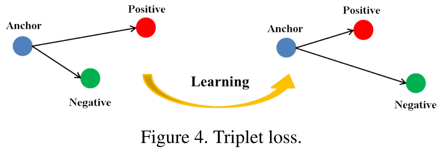



损失函数为：

L=∑Nmax{∥∥f(xa)−f(xp)∥∥22+α−∥∥f(xa)−f(xn)∥∥22, 0}

Triplet Loss 中 margin 取值分析

我们的目的就是使 loss 在训练迭代中下降的越小越好，也就是要使得 Anchor 与 Positive 越接近越好，Anchor 与 Negative 越远越好。基于上面这些，分析一下 margin 值的取值。

当 margin 值越小时，loss 也就较容易的趋近于 0，于是 Anchor 与 Positive 都不需要拉的太近，Anchor 与 Negative 不需要拉的太远，就能使得 loss 很快的趋近于 0。这样训练得到的结果，不能够很好的区分相似的图像。

当 Anchor 越大时，就需要使得网络参数要拼命地拉近 Anchor、Positive 之间的距离，拉远 Anchor、Negative 之间的距离。如果 margin 值设置的太大，很可能最后 loss 保持一个较大的值，难以趋近于 0 。

因此，设置一个合理的 margin 值很关键，这是衡量相似度的重要指标。简而言之，margin 值设置的越小，loss 很容易趋近于 0 ，但很难区分相似的图像。margin 值设置的越大，loss 值较难趋近于 0，甚至导致网络不收敛，但可以较有把握的区分较为相似的图像。

Triplet Loss 实验1

分析完了，就得通过实验来验证。

当我在 Triplet Loss 中的 Model 设置为 VGG Net 。同时，margin = 0.2，才跑没几下，这个 Loss 曲线就诡异的先猛的增大，之后突然降为 0 了。不知道为何？如下：



我的猜想是，VGG Net 本身是很深的网络，但网络一深，到最后提取到的特征向量就很深。相似图像之间，更多的细节在卷积网络层中被层层过滤掉了。到最后两张相似图像之间特征区别不大了，即使将 margin 设置为 0.2，这么比较小的数值，也不行。

Triplet Loss 实验2

同样的数据，margin ＝ 0.2，对于不同的网络，如下面的这个 AlexNet 网络（有改动）：

-----------------------------------------------------------
-- Network definition --
-----------------------------------------------------------
backend = nn

convNet = nn.Sequential()
convNet:add(backend.SpatialConvolution(3,64, 3,3, 1,1, 1,1))
convNet:add(backend.ReLU(true)):add(nn.Dropout(0.3))
convNet:add(backend.SpatialMaxPooling(2, 2, 2, 2):ceil())

convNet:add(backend.SpatialConvolution(64, 128, 3,3, 1,1, 1,1))
convNet:add(backend.ReLU(true)):add(nn.Dropout(0.4))
convNet:add(backend.SpatialMaxPooling(2, 2, 2, 2):ceil())

convNet:add(backend.SpatialConvolution(128, 256, 3,3, 1,1, 1,1))
convNet:add(backend.ReLU(true)):add(nn.Dropout(0.4))
convNet:add(backend.SpatialMaxPooling(2, 2, 2, 2):ceil())

convNet:add(backend.SpatialConvolution(256, 512, 3,3, 1,1, 1,1))
convNet:add(backend.ReLU(true)):add(nn.Dropout(0.5))
convNet:add(backend.SpatialMaxPooling(2, 2, 2, 2):ceil())

convNet:add(backend.SpatialConvolution(512, 512, 3,3, 1,1, 1,1))
convNet:add(backend.ReLU(true)):add(nn.Dropout(0.5))
convNet:add(backend.SpatialMaxPooling(2, 2, 2, 2):ceil())

convNet:add(nn.View(512*4*4))

convNet:add(nn.Linear(512*4*4, 4096*4))
convNet:add(nn.ReLU(true))
convNet:add(nn.Dropout(0.5))
convNet:add(nn.Linear(4096*4, 4096))
convNet:add(nn.ReLU(true))
convNet:add(nn.Dropout(0.5))
convNet:add(nn.Linear(4096, 1024))

-- initialization from MSR
local function MSRinit(net)
local function init(name)
for k, v in pairs(net:findModules(name)) do
local n = v.kW * v.kH * v.nOutputPlane
v.weight:normal(0, math.sqrt(2/n))
v.bias:zero()
end
end
-- have to do for both backends
init'cudnn.SpatialConvolution'
init'nn.SpatialConvolution'
end
MSRinit(convNet)

convNetPos = convNet:clone('weight', 'bias', 'gradWeight', 'gradBias')
convNetNeg = convNet:clone('weight', 'bias', 'gradWeight', 'gradBias')

-- Parallel container
parallel = nn.ParallelTable()
parallel:add(convNet)
parallel:add(convNetPos)
parallel:add(convNetNeg)

parallel = parallel:cuda()

parameters, gradParameters = parallel:getParameters()

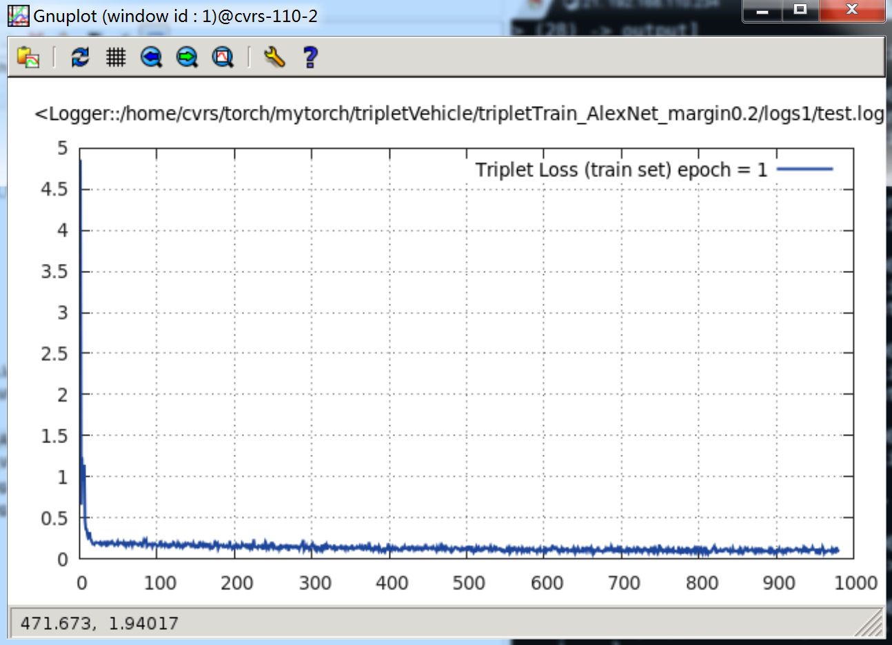
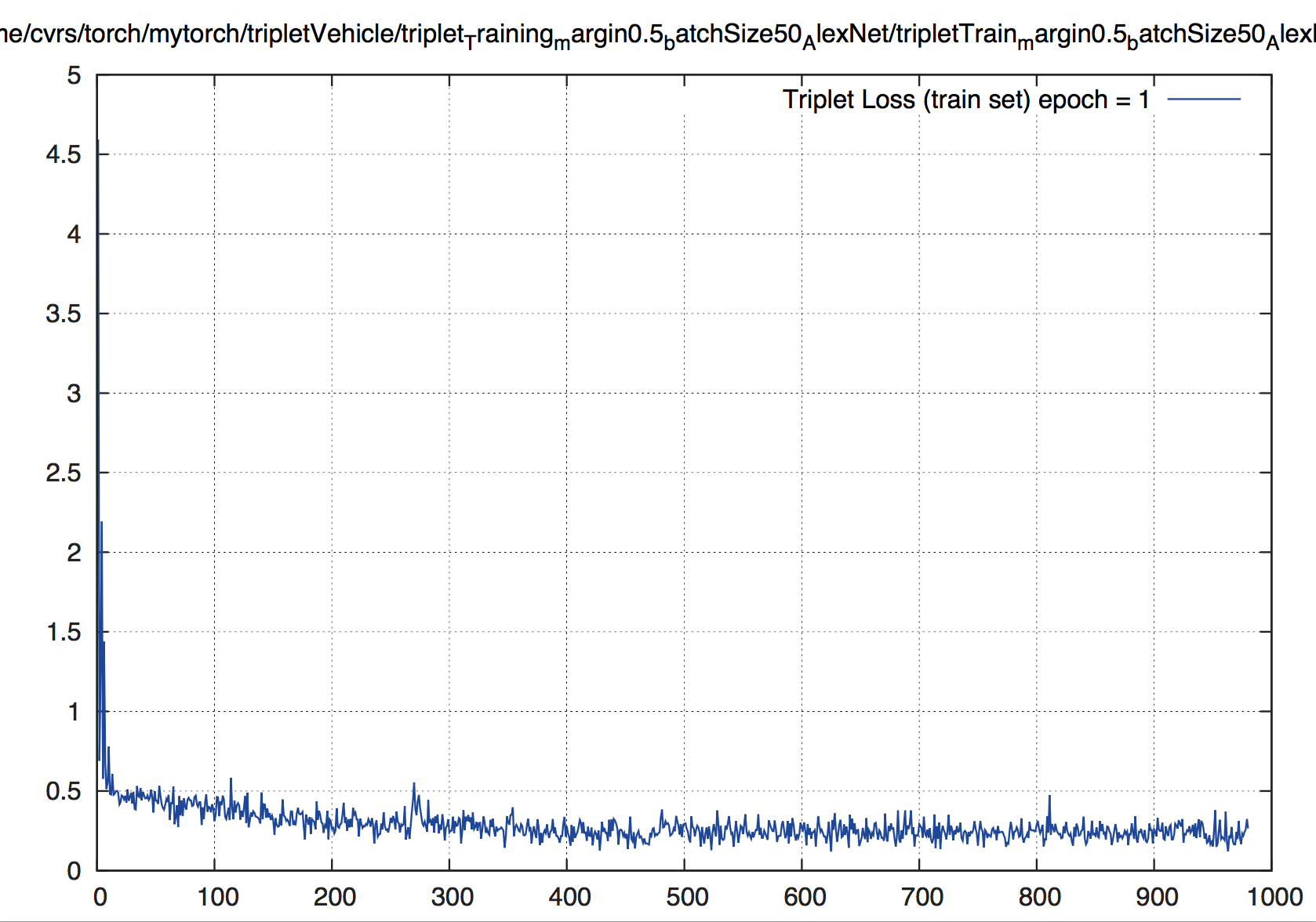
print(b('Fresh-embeddings-computation network:')); print(parallel)

上面这个较浅的网络，就很快收敛了。当

epoch = 1

时，Loss 曲线如下：



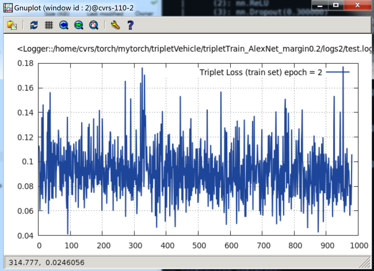
当

epoch = 2

时，Loss 曲线如下：



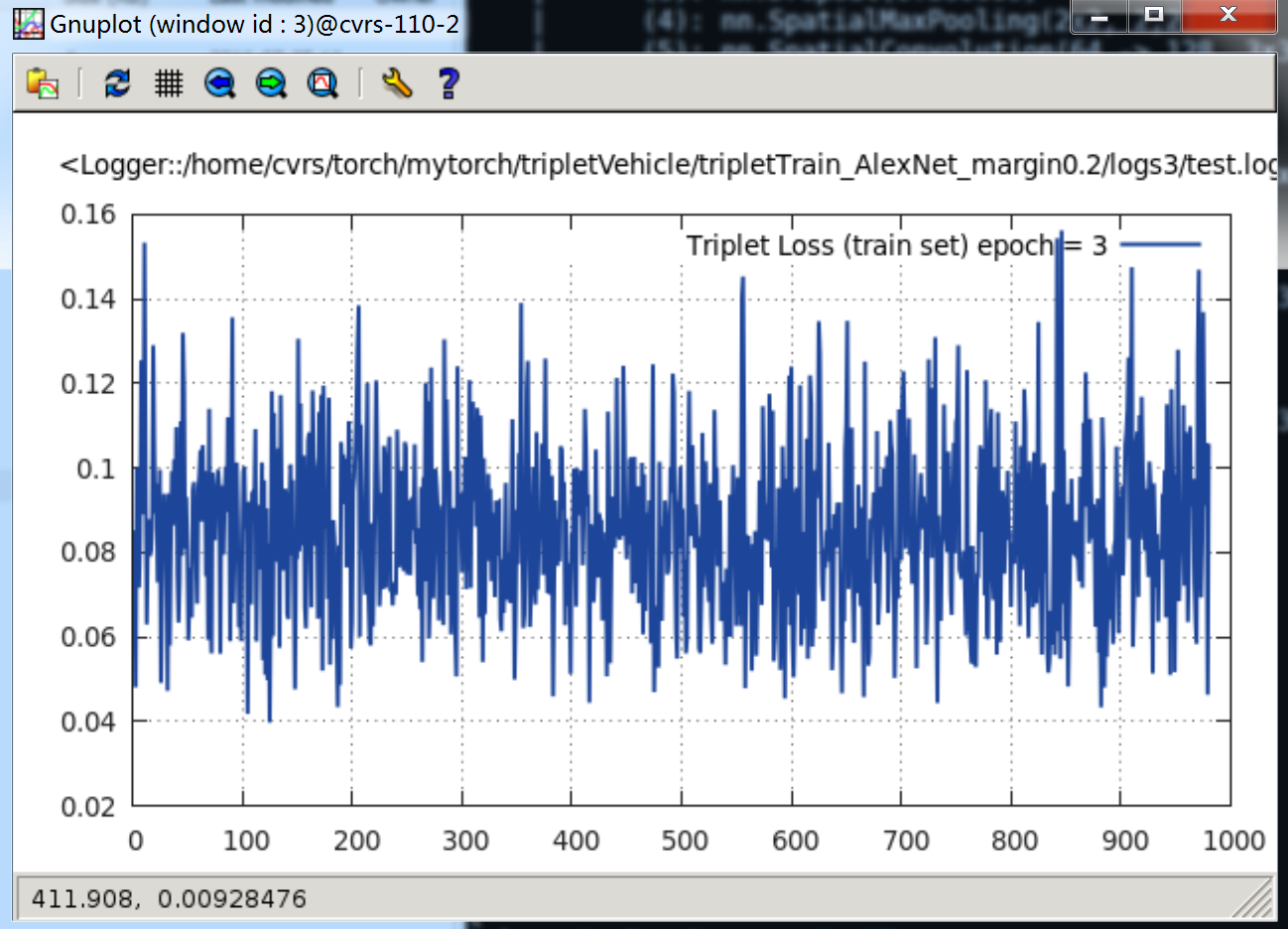
当

epoch = 3

时，Loss 曲线如下：



最后，当

epoch = 100

时，Loss 曲线如下：



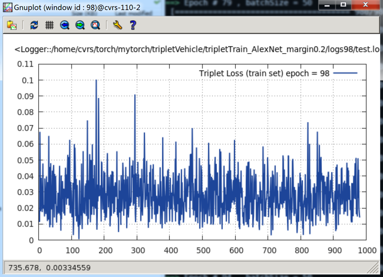
可以看见，最后这个 loss 下降到 0.01 ~ 0.03 之间，其实这还有点大。

Triplet Loss 实验3

下面，当 margin 值设置为 0.5 时，

epoch = 1

时，loss 曲线如下：

epoch = 2

时，loss 曲线如下：



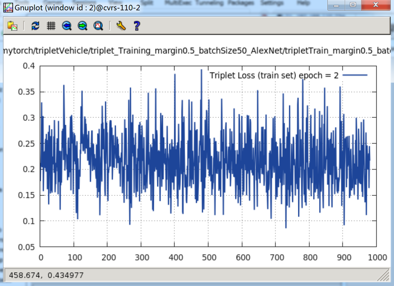
当

epoch = 16

时，loss 曲线如下：



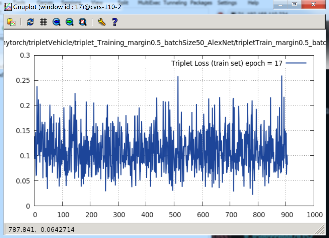
当

epoch = 17

时，loss 曲线如下：



当

epoch = 28

时，loss 曲线如下：



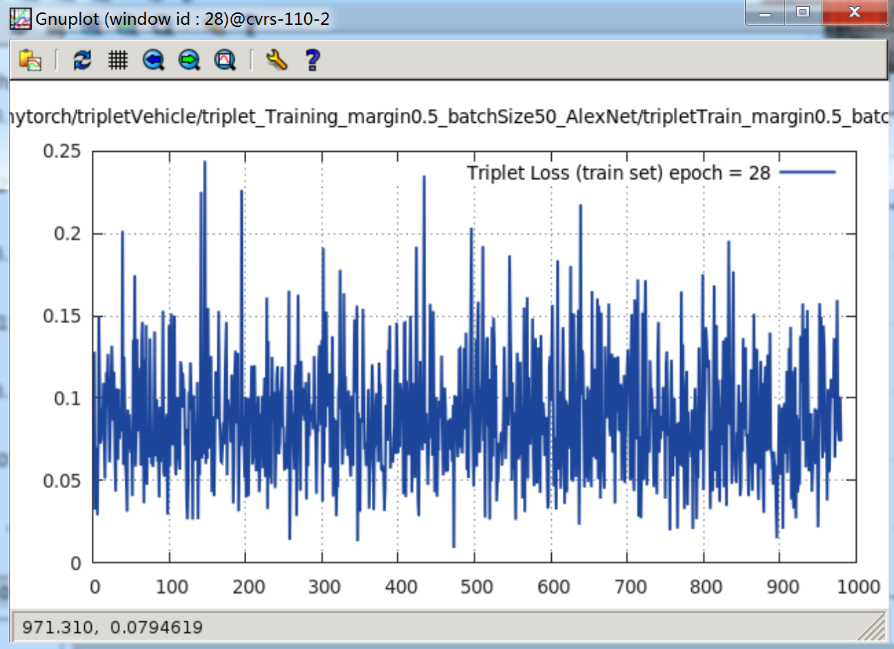
可以看见，其 Loss 一直在下降。

当 margin ＝ 0.2 时，很快的便能下降到 0.1 附近，接着跑一天一夜，loss 便下降到 0.01 ~ 0.03 附近。

当 margin = 0.5 时，很快的便能下降到 0.2 ~ 0.25 附近。接着再跑，loss 就慢慢再下降，经过 17 个纪元，就下降到了 0.1 ~ 0.15 附近。还会进一步下降。

用训练好的 model 进行 predict 测试

这里我折腾了一晚，有点……诡异……我将训练好的模型加载后，传入数据，无论我输入什么 Tensor，模型输出 predict 居然都是一样的值……这里把我郁闷了半天。

下面是我用测试图片（Anchor 5 张图像、Positive 5 张图像、Negative 5 张图像）进行模型的测试代码：

require 'nn'
require 'image'
require 'paths'
require 'cunn'
require 'cudnn'

-------------------------------------------------------------
-- load images
-- aImgs: Anchor, pImgs: Positive, nImgs: Negative
-------------------------------------------------------------
aImgs = torch.Tensor(5, 3, 128, 128)
local aImgs_i = 1
for f in paths.iterfiles('tripletTestImgs/aImgs/') do
local img = image.load('tripletTestImgs/aImgs/' .. f)
aImgs[aImgs_i] = image.scale(img, 128, 128)
aImgs_i = aImgs_i + 1
end

pImgs = torch.Tensor(5, 3, 128, 128)
local pImgs_i = 1
for f in paths.iterfiles('tripletTestImgs/pImgs/') do
local img = image.load('tripletTestImgs/pImgs/' .. f)
pImgs[pImgs_i] = image.scale(img, 128, 128)
pImgs_i = pImgs_i + 1
end

nImgs = torch.Tensor(5, 3, 128, 128)
local nImgs_i = 1
for f in paths.iterfiles('tripletTestImgs/nImgs/') do
local img = image.load('tripletTestImgs/nImgs/' .. f)
nImgs[nImgs_i] = image.scale(img, 128, 128)
nImgs_i = nImgs_i + 1
end

-------------------------------------------------------------
-- load trained model
-- margin  = 0.2, batchSize = 50, Net = AlexNet
-------------------------------------------------------------
model = torch.load('model_AlexNet.t7')
print(model.modules[1])
print(model.modules[2])
print(model.modules[3])

predict1 = model.modules[1]:forward(aImgs:cuda())
predict2 = model.modules[1]:forward(pImgs:cuda())
predict3 = model.modules[1]:forward(nImgs:cuda())

print('\n---------------------------------------------- \n')
dist1 = torch.sum(torch.cmul(predict1 - predict2, predict1 - predict2), 2)
print('dist1: ');print(dist1)

print('\n----------------------------------------------')
dist2 = torch.sum(torch.cmul(predict1 - predict2, predict1 - predict2), 2)
print('dist2: ');print(dist2)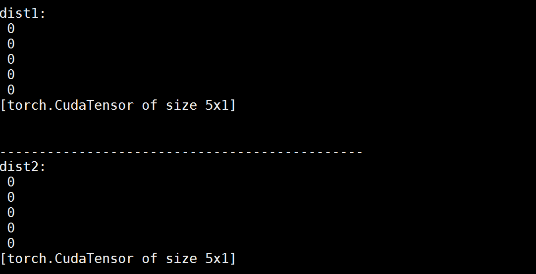

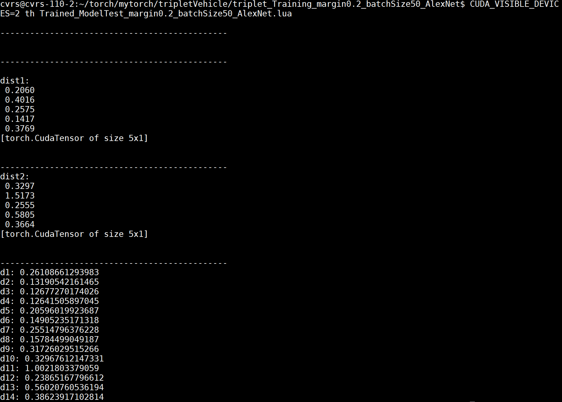
当我把预测部分的代码改成如下：

predict = model:forward({aImgs:cuda(), pImgs:cuda(), nImgs:cuda()})

print('\n---------------------------------------------- \n')
dist1 = torch.sum(torch.cmul(predict[1] - predict[2], predict[1] - predict[2]), 2)
print('dist1: ');print(dist1)

print('\n----------------------------------------------')
dist2 = torch.sum(torch.cmul(predict[1] - predict[3], predict[1] - predict[3]), 2)
print('dist2: ');print(dist2)

print('\n----------------------------------------------')
d1 = torch.sum(torch.cmul(predict[1][1] - predict[1][2], predict[1][1] - predict[1][2]))
print('d1: ' .. d1)

d2 = torch.sum(torch.cmul(predict[1][1] - predict[1][3], predict[1][1] - predict[1][3]))
print('d2: ' .. d2)

d3 = torch.sum(torch.cmul(predict[1][1] - predict[1][4], predict[1][1] - predict[1][4]))
print('d3: ' .. d3)

d4 = torch.sum(torch.cmul(predict[1][1] - predict[1][5], predict[1][1] - predict[1][5]))
print('d4: ' .. d4)

d5 = torch.sum(torch.cmul(predict[1][1] - predict[2][1], predict[1][1] - predict[2][1]))
print('d5: ' .. d5)

d6 = torch.sum(torch.cmul(predict[1][1] - predict[2][2], predict[1][1] - predict[2][2]))
print('d6: ' .. d6)

d7 = torch.sum(torch.cmul(predict[1][1] - predict[2][3], predict[1][1] - predict[2][3]))
print('d7: ' .. d7)

d8 = torch.sum(torch.cmul(predict[1][1] - predict[2][4], predict[1][1] - predict[2][4]))
print('d8: ' .. d8)

d9 = torch.sum(torch.cmul(predict[1][1] - predict[2][5], predict[1][1] - predict[2][5]))
print('d9: ' .. d9)

d10 = torch.sum(torch.cmul(predict[1][1] - predict[3][1], predict[1][1] - predict[3][1]))
print('d10: ' .. d10)

d11 = torch.sum(torch.cmul(predict[1][1] - predict[3][2], predict[1][1] - predict[3][2]))
print('d11: ' .. d11)

d12 = torch.sum(torch.cmul(predict[1][1] - predict[3][3], predict[1][1] - predict[3][3]))
print('d12: ' .. d12)

d13 = torch.sum(torch.cmul(predict[1][1] - predict[3][4], predict[1][1] - predict[3][4]))
print('d13: ' .. d13)

d14 = torch.sum(torch.cmul(predict[1][1] - predict[3][5], predict[1][1] - predict[3][5]))
print('d14: ' .. d14)

就有值了：



但奇怪的是，输出的值，每次运行都不一样，如过我再运行一次，就会变成下面的值：



经过 Google，终于找到每次输入，输出的值不一样的原因了！原来是我在网络中加了 Dropout 层，在这个 Torch 的文档中找到了解释：

In this example, we demonstrate how the call to forward samples different

outputs

to dropout (the zeros) given the same

input

:

module = nn.Dropout()

> x = torch.Tensor{{1, 2, 3, 4}, {5, 6, 7, 8}}

> module:forward(x)
2   0   0   8
10   0  14   0
[torch.DoubleTensor of dimension 2x4]

> module:forward(x)
0   0   6   0
10   0   0   0
[torch.DoubleTensor of dimension 2x4]

Triplet Loss 实验4

看来得把 Dropout 的那篇 2014 年 JMLR 的 Paper 《Dropout - A Simple Way to Prevent Neural Networks from Overfitting》 看一下了～

于是我干脆将上面网络中的 Dropout 层取消掉，看实验效果。同时参数设置：

margin = 0.5

，

batchSize = 50

，取消之后的网络为：

-----------------------------------------------------------
-- Network definition --
-- Cut out the Dropout Layer --
-----------------------------------------------------------
backend = nn

convNet = nn.Sequential()
convNet:add(backend.SpatialConvolution(3,64, 3,3, 1,1, 1,1))
convNet:add(backend.ReLU(true))
convNet:add(backend.SpatialMaxPooling(2, 2, 2, 2):ceil())

convNet:add(backend.SpatialConvolution(64, 128, 3,3, 1,1, 1,1))
convNet:add(backend.ReLU(true))
convNet:add(backend.SpatialMaxPooling(2, 2, 2, 2):ceil())

convNet:add(backend.SpatialConvolution(128, 256, 3,3, 1,1, 1,1))
convNet:add(backend.ReLU(true))
convNet:add(backend.SpatialMaxPooling(2, 2, 2, 2):ceil())

convNet:add(backend.SpatialConvolution(256, 512, 3,3, 1,1, 1,1))
convNet:add(backend.ReLU(true))
convNet:add(backend.SpatialMaxPooling(2, 2, 2, 2):ceil())

convNet:add(backend.SpatialConvolution(512, 512, 3,3, 1,1, 1,1))
convNet:add(backend.ReLU(true))
convNet:add(backend.SpatialMaxPooling(2, 2, 2, 2):ceil())

convNet:add(nn.View(512*4*4))

convNet:add(nn.Linear(512*4*4, 4096*4))
convNet:add(nn.ReLU(true))
convNet:add(nn.Linear(4096*4, 4096))
convNet:add(nn.ReLU(true))
convNet:add(nn.Linear(4096, 1024))

-- initialization from MSR
local function MSRinit(net)
local function init(name)
for k, v in pairs(net:findModules(name)) do
local n = v.kW * v.kH * v.nOutputPlane
v.weight:normal(0, math.sqrt(2/n))
v.bias:zero()
end
end
-- have to do for both backends
init'cudnn.SpatialConvolution'
init'nn.SpatialConvolution'
end
MSRinit(convNet)

convNetPos = convNet:clone('weight', 'bias', 'gradWeight', 'gradBias')
convNetNeg = convNet:clone('weight', 'bias', 'gradWeight', 'gradBias')

-- Parallel container
parallel = nn.ParallelTable()
parallel:add(convNet)
parallel:add(convNetPos)
parallel:add(convNetNeg)

parallel = parallel:cuda()
parameters, gradParameters = parallel:getParameters()
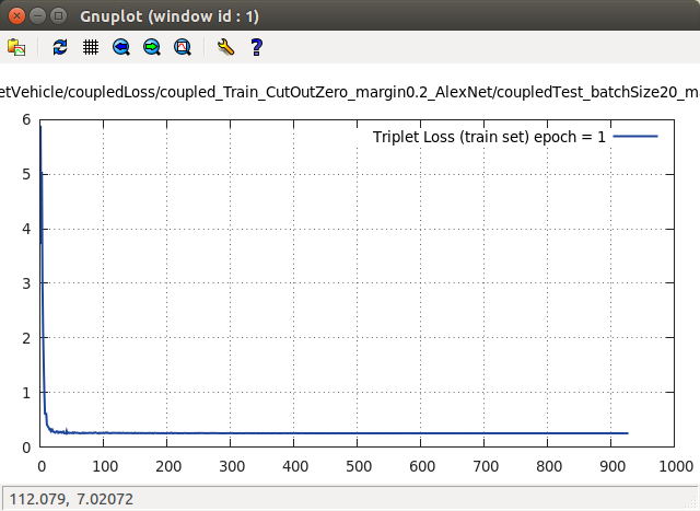
print(b('Fresh-embeddings-computation network:')); print(parallel)

当

epoch = 1

时，其 loss 曲线为：



当

epoch = 2

时，其 loss 曲线为：



当

epoch =

时，其 loss 曲线为：



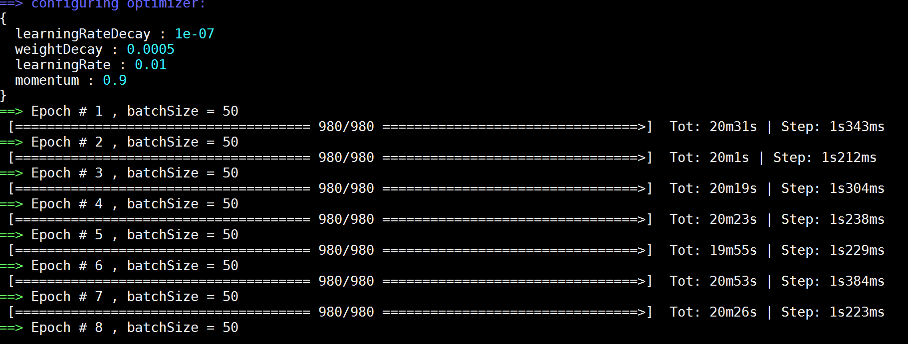
突然发现没有了 Dropout 层，训练的 loss 收敛速度要远远快于有 Dropout 层。但同时，每一个 epoch 的速度消耗时间也变长了，是有 Dropout 层所消耗时间的 3 ~ 4 倍：



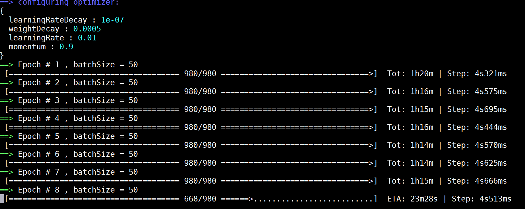
看有 Dropout 层的训练时间消耗：

Coupled Cluster Loss

Coupled Cluster Loss 的 Torch 实现

当我将 Triplet Loss 改写为 Coupled Cluster Loss，其损失函数模块的代码如下，这改写没什么难的，依葫芦画瓢就好了：

------------------------------------------
-- Coupled Cluster Loss --
-- Xinpeng.Chen --
------------------------------------------

local CoupledClusterLoss, parent = torch.class('nn.CoupledClusterLoss', 'nn.Criterion')

function CoupledClusterLoss:__init(alpha)
parent.__init(self)
self.alpha = alpha or 0.2 -- margin
self.Li = torch.Tensor()
self.gradInput = {}
end

function CoupledClusterLoss:updateOutput(input)
local p = input[1] -- p is the 5 * 1024 vector
local n = input[2] -- n is the 5 * 1024 vector
local N = p:size(1)

-- find the center of the positive points
local centerP = torch.sum(p, 1) / N

-- fing the closest negative vector to the centerP
local negToCP = torch.Tensor(N)

for i = 1, N do
negToCP[i] = torch.sum( torch.cmul(centerP - n[i], centerP - n[i]) )
end
local minNegToCP, minIndex = torch.min(negToCP, 1)

-- Caculate the loss
self.Li:resize(N)
for j = 1, N do
-- self.Li[j] = 0.5 * math.max(0, torch.sum( torch.cmul(p[i] - centerP, p[i] - centerP) ) + self.alpha - torch.sum( torch.cmul(n[minIndex[1]] - centerP, n[minIndex[1]] - centerP) ) )
self.Li[j] = 0.5 * math.max( 0, (p[j] - centerP) * (p[j] - centerP) + self.alpha - (n[minIndex[1]] - centerP) * (n[minIndex[1]] - centerP) )
end

self.output = self.Li:sum()

return self.output
end

function CoupledClusterLoss:updateGradInput(input)
local p = input[1] -- p is the 5 * 1024 vector
local n = input[2] -- n is the 5 * 1024 vector
local N = p:size(1)

-- find the center of the positive points
local centerP = torch.sum(p, 1) / N

-- fing the closest negative vector to the centerP
local negToCP = torch.Tensor(N)

for i = 1, N do
negToCP[i] = torch.sum( torch.cmul(centerP - n[i], centerP - n[i]) )
end
local minNegToCP, minIndex = torch.min(negToCP, 1)

-- Caculate the gradient of input
if torch.type(p) == 'torch.CudaTensor' then -- if buggy CUDA API
self.gradInput[1] = (p - centerP:repeatTensor(N, 1)):cmul(self.Li:gt(0):repeatTensor(p:size(2), 1):type(p:type()) )
self.gradInput[2] = (centerP:repeatTensor(N, 1) - n[minIndex[1]]:repeatTensor(N, 1)):cmul(self.Li:gt(0):repeatTensor(p:size(2), 1):type(p:type()) )
else
self.gradInput[1] = self.Li:gt(0):diag():type(p:type()) * (p - centerP:repeatTensor(N, 1))
self.gradInput[2] = self.Li:gt(0):diag():type(p:type()) * (centerP:repeatTensor(N, 1) - n[minIndex[1]]:repeatTensor(N, 1))
end

return self.gradInput
end

Coupled Cluster Loss 的示意图 及其 Loss Function

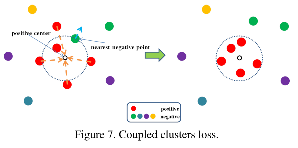
L(W,Xp,Xn)=∑iNp12max{0, ∥∥f(xpi)−cp∥∥22+α−∥∥f(xn∗)−cp∥∥22}

Coupled Cluster Loss 中 margin 取值分析

一开始我比较疑惑，这个 margin 值该怎样设置呢？下面是我的分析：

我们的目标是尽量使得 loss 下降到 0，在迭代梯度更新的过程中，要使得第一项：∥∥f(xpi)−cp∥∥22 尽可能的小，即在图中就是使得相似图片与其中心的距离越小越好，而与中心最近的负样本之距离越大越好。

当 margin，即公式中的 α 越大时，就要使得正样本与中心的距离更小，离中心最近的负样本与中心之距离越大，才能使得 loss 将为 0 。

当 margin 越小时，比如设置为 0.05 或者直接是 0 时，正样本与中心的距离就没有必要像 margin 较大时的那样，拼命的”靠在一起”才能使得 loss 为 0，负样本也没必要尽量的与中心”拉远”距离了。

所以，通过上面的分析，这个 margin 很关键。设置的太小，如 0，那么 loss 很容易就下降到 0，因为正样本与中心的距离本应就小于最近负样本与中心的距离。如果设置的太大，那么就很难收敛了，因为无论网络的梯度怎么更新，即使正样本与中心都重合了，最近负样本与中心的距离要”拉得”很远才有可能使得 loss 将为 0 。

Coupled Cluster Loss 实验1

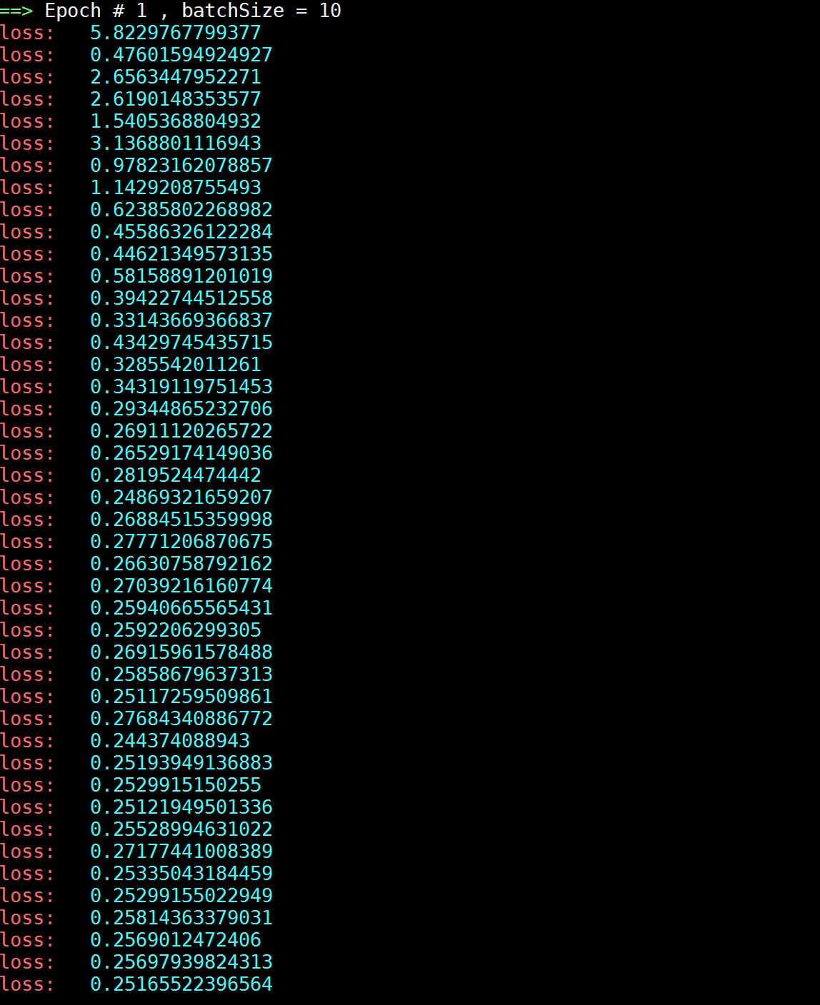
当 Net 为 AlexNet，Margin = 0.5，batchSize = 10 。

在第一个纪元，即 epoch ＝ 1 时，其 loss 曲线（因为 trainSize = 49000，所以在一个 epoch 内，共有 4900 次计算迭代，下图只是一部分）：



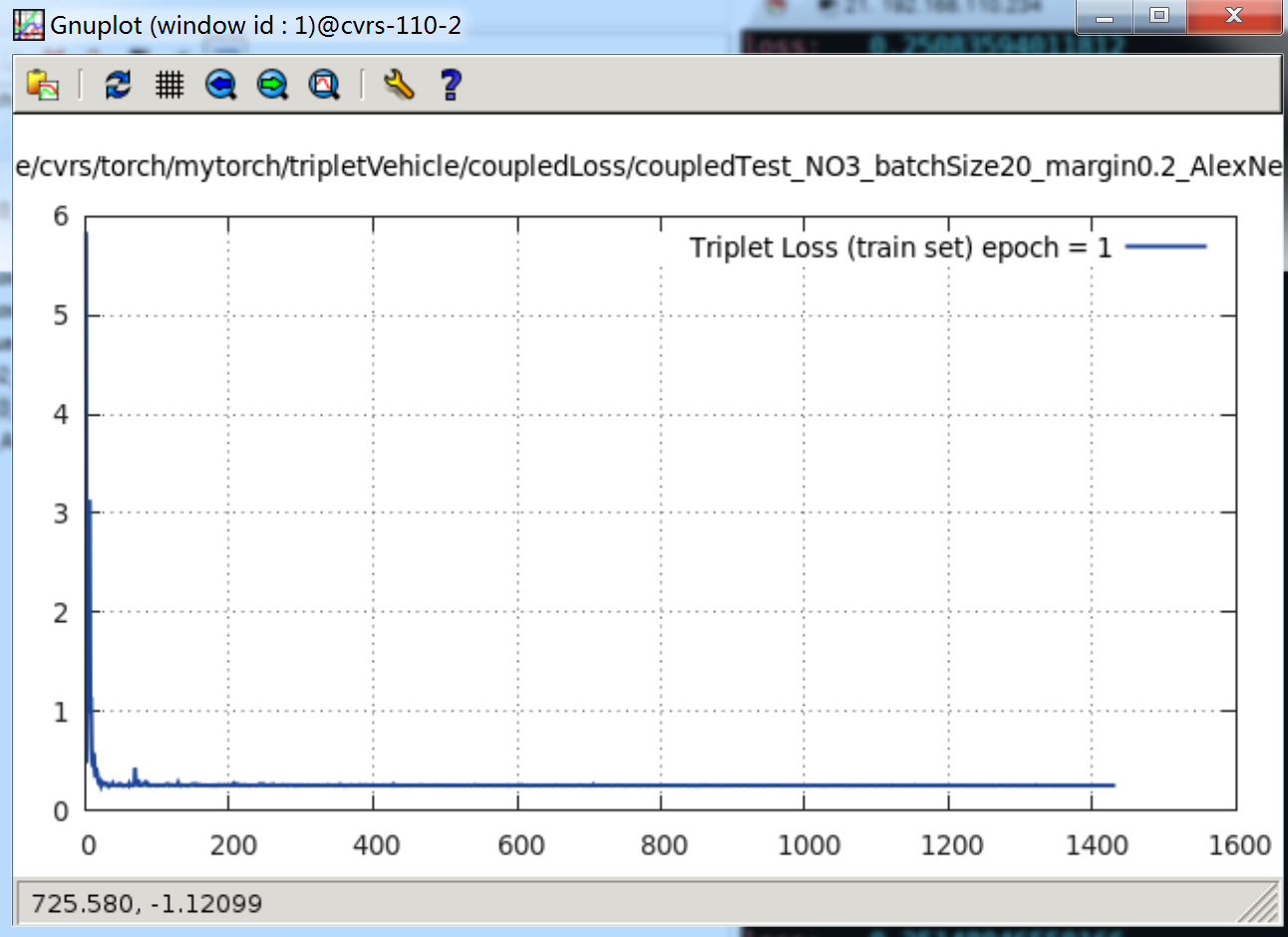
可以看见，loss 很快下降到 0.25 的位置上就很难往下降了。我将 loss 打印出来：



下图是跑了一个晚上，跑到当

epoch = 18

时的情况：



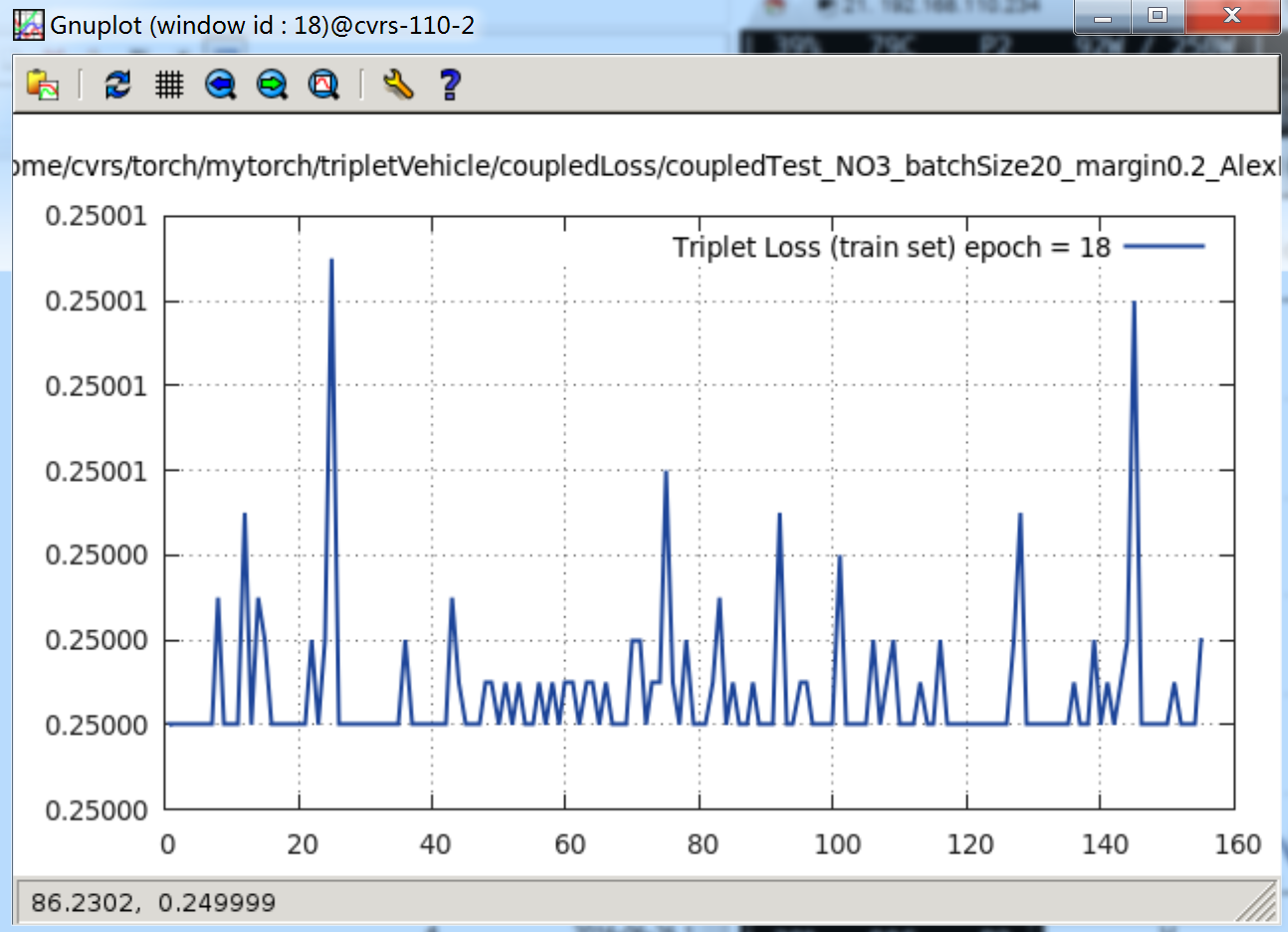
是不是比上面的 Triplet Loss 诡异？就只到 0.25，之后就不再往下降一点点了。

Coupled Cluster Loss 实验2

我开始找原因，是什么导致了这种情况？我注意到，当 margin 取值 0.5 的时候，结合其 loss 函数：

L(W,Xp,Xn)=∑iNp12max{0, ∥∥f(xpi)−cp∥∥22+α−∥∥f(xn∗)−cp∥∥22}

0.25 正好是 12×margin，margin 取值 为 0.5。所以，我开始怀疑这篇论文中所提到的 Coupled Cluster Loss 到底合不合适，正不正确？

这时候我将上面损失函数改写一下，就是去掉公式中和 0 的比较：：

L(W,Xp,Xn)=∑iNp12( ∥∥f(xpi)−cp∥∥22+α−∥∥f(xn∗)−cp∥∥22 )

但实验结果依然如此，loss 还是降到 0.25 就降不下去：



打印出 loss 如下：

Coupled Cluster Loss 实验3

当我的 margin = 1 时，其 loss 还只是下降到一半就不下了：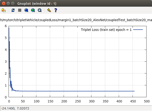

Coupled Cluster Loss 实验4

到这里，我先断了训练，改变 margin 值试试看，我将 margin 改为 0.05 时，其 loss 走势如下：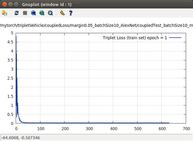



打印出来如下：





从上面可以看见，当 margin = 0.05 时，其 loss 就下降到 0.025 。因此，是不是发现了一个规律？loss 最后的底线值是 margin 值的一半。

Coupled Cluster Loss 实验5

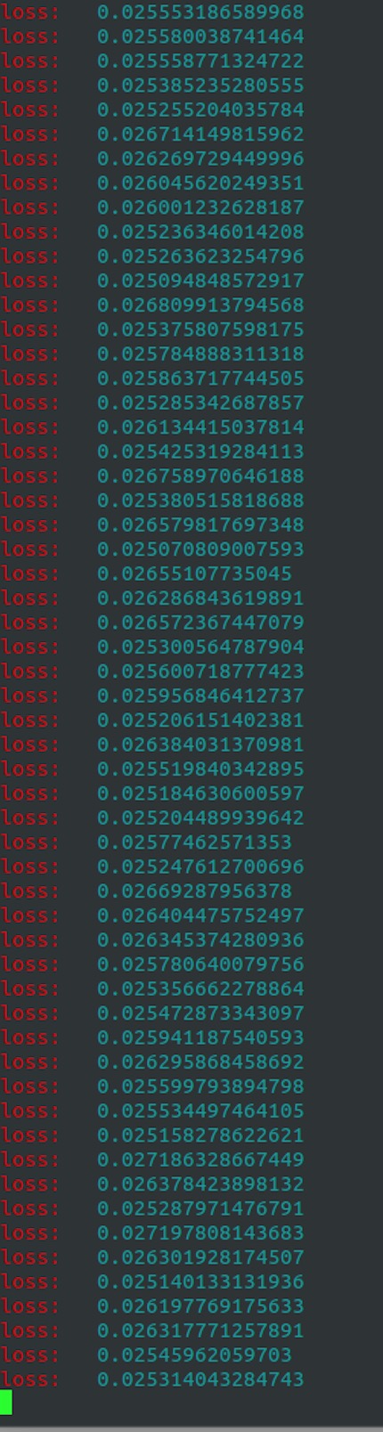
当 margin ＝ 0.01 时，那就是只下降到 0.05，其 loss 曲线如下：

当

epoch = 3

时，



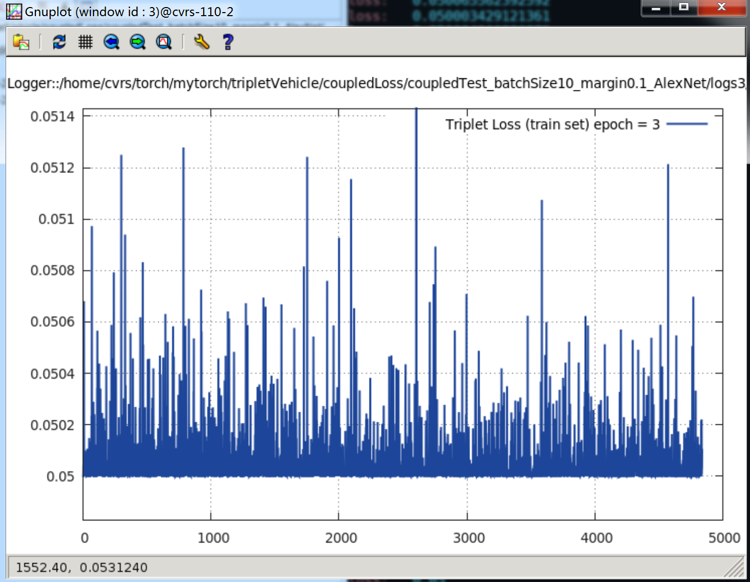
当

epoch = 4

时，



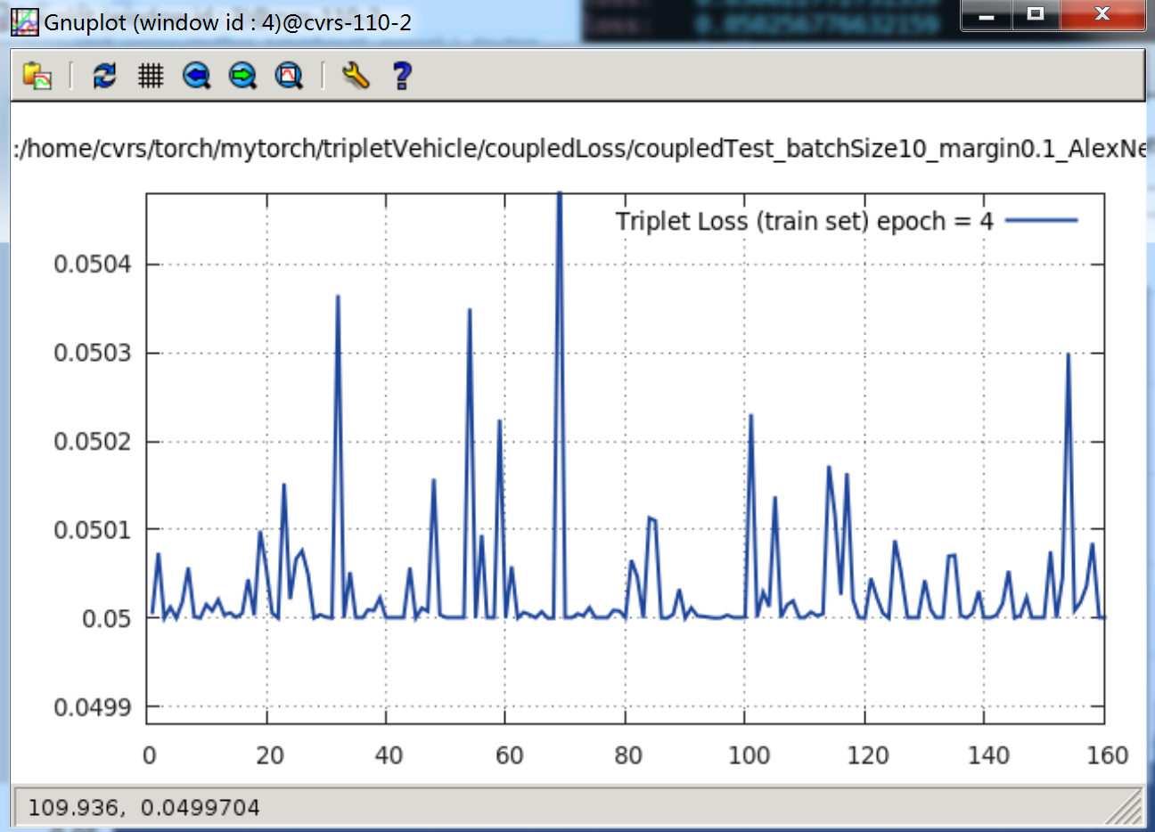
看 Terminal 打印出来的内容就更清楚了，只到 0.05，就再不肯往下降一点：

Coupled Cluster Loss 实验发现与猜想、分析

根据上面的实验，所以我猜想 margin 取值与 loss 之间有如下关系：



为什么会这样，我想想，这或许与数据有关系。

几个正样本就很接近，所以损失函数的第一项就几乎为 0，第二项是 margin 的值 α，第三项就是 到中心距离最近的负样本之距离。其实第三项，我想也很接近于 0，因为经过网络的训练，负样本的特征向量与正样本的特征向量差别并不大，都是车，在很难区分的细节上有些差异。