R语言 ETL+统计+可视化

setwd("C:/Users/liyi/Desktop")
a<-readLines("message2.txt",encoding = "UTF-8",skipNul=T)
head(a,20)
nchar(a)
# 除去空白行
newa<-a[nchar(a)>1]
length(a)
length(newa)
head(newa,10)
#删除前6行
newa1<-newa[7:length(newa)]
head(newa1,10)
#寻找发言人 “2016-04-23 21:26:02 (qq-xxxxxxxxx)”
temp<-grep("2016-.",newa1);temp
time_name_qq<-newa1[temp]
#防止有人更换昵称，将QQ号作为唯一的标识
str(time_name_qq)

head(time_name_qq)
[1] "2016-04-23 21:26:02 (4xxxxxxxx)"              "2016-04-23 21:26:22 xxxxx(xxxxxxx)"
[3] "2016-04-23 21:26:54 (4xxxxxxxxx)"              "2016-04-23 21:51:21 Fair(1xxxxxxxxx)"
[5] "2016-04-23 22:39:02 麦x(1xxxxxxxxx7)"         "2016-04-24 9:13:45 (xxxxxxxx)"

经观察，time_name_qq 的格式，QQ号 位于（）或者<> 内，截取QQ号，利用正则表达式

subqq<-function(x){
start<-regexpr("\\(|<",x)
end<-regexpr("\\)|>",x)
substr(x,start+1,end-1)
}
qq<-subqq(time_name_qq)

计算每次留言的行数
liuyan<-c(1:length(temp))

for (i in 1:length(temp)){
liuyan[i] <-(temp[i+1]-temp[i])
}
liuyan<-liuyan-1
liuyan[length(temp)]<-1

QQ号按留言行数重现
totalqq<-rep(qq,liuyan)
totalqq
tb_qq<-table(totalqq)
tb_qq<-as.data.frame.table(tb_qq)

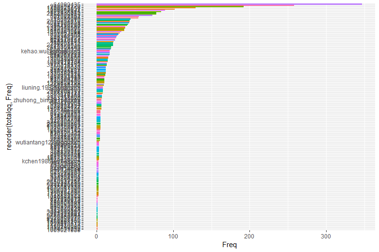
按留言量将tb_qq结果可视化
plot_qq<-ggplot(tb_qq)+geom_bar(aes(x=reorder(totalqq,Freq),y=Freq,fill=totalqq),stat = "identity")+
coord_flip()+
theme(legend.position='none')

查看每人留言情况的分布

hist_qq<-ggplot(tb_qq,aes(x=Freq,fill=..x..))+geom_histogram(binwidth = 2)

box_qq<-ggplot(tb_qq,aes(x="totalqq",y=Freq))+geom_boxplot()+geom_jitter()
library(grid)
subvp<-viewport(width = 0.4,height = 0.5,x=0.7,y=0.75)
hist_qq
print(box_qq,vp=subvp)

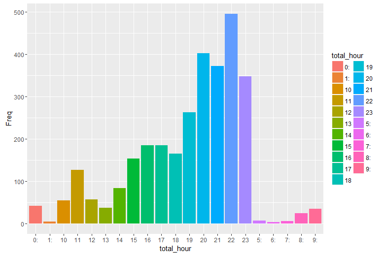
查看一天各时段留言量分布情况
time<-substr(time_name_qq,1,19)
head(time)
total_time<-rep(time,liuyan)
total_hour<-rep(substr(time_name_qq,12,13),liuyan)

tb_hour<-table(total_hour)
tb_hour<-as.data.frame.table(tb_hour)

hour<-ggplot(tb_hour)+
geom_bar(aes(x=total_hour,y=Freq,fill=total_hour),stat = "identity")
hour

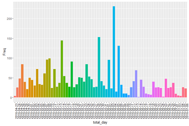
查看留言量按天的分布
total_day<-rep(substr(time_name_qq,1,10),liuyan)
tb_day<-table(total_day)
tb_day<-as.data.frame.table(tb_day)

day<-ggplot(tb_day)+geom_bar(aes(x=total_day,y=Freq,fill=total_day),stat = "identity")+
theme(axis.text.x=element_text(angle=90,hjust=1,colour="black"),legend.position='none')
day

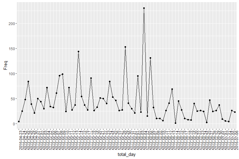
day<-ggplot(tb_day,aes(x=total_day,y=Freq,group=1))+
geom_point()+geom_path()+
theme(axis.text.x=element_text(angle=90,hjust=1,colour="black"),legend.position='none')
day