Lesson 2 Gradient Desent

The goal is to find X such that minXf(X)

Using gradient descent algorithm to obtain the minimum value of the funtion.

let y=f(x)

Init: x=x0,y0=f(x0), iterative step α, convergent precision ϵ

The ith iterative formula can be expressed as:

xi=xi−1−α∇f(xi−1)

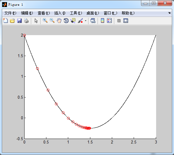
Example: solve the minimum of function f(x)=x2+3x+2

let x0=0, step \alpha = 0.1, convergent precision ϵ=10−4

f = @(x) x.^2 - 3*x + 2;
hold on
for x=0:0.001:3
plot(x, f(x),'k-');
end

x = 0;
y0 = f(x);
plot(x, y0, 'ro-');
alpha = 0.1;
epsilon = 10^(-4);

gnorm = inf;

while (gnorm > epsilon)
x = x - alpha*(2*x-3);
y = f(x);
gnorm = abs(y-y0);
plot(x, y, 'ro');
y0 = y;
end

let’s move into multi-variable case, say we have m samples, each sample has n features. X is expressed as: X=⎡⎣⎢⎢⎢⎢⎢xT1xT2⋮xTm⎤⎦⎥⎥⎥⎥⎥

where

xi=⎡⎣⎢⎢⎢⎢xi1xi2⋮xin⎤⎦⎥⎥⎥⎥

Then X can be denoted as :

X=⎡⎣⎢⎢⎢⎢⎢x11x21⋮xm1x11x21⋮xm1⋯⋯⋱⋯x1nx2n⋮xmn⎤⎦⎥⎥⎥⎥⎥

Assuming h(x.)=∑j=1najx.j=xT.a

Here, a=⎡⎣⎢⎢⎢⎢a1a2⋮an⎤⎦⎥⎥⎥⎥ is a unknown vector we need to solve.

Xa−y=⎡⎣⎢⎢⎢⎢⎢h(x1)−y1h(x2)−y2⋮h(xm)−ym⎤⎦⎥⎥⎥⎥⎥

Now the objective function is minaf(a)=12(Xa−y)T(Xa−y)

Before the derivation, I would like to introduce some facts:

tr(AB)=tr(BA) ………………………………..(1)

tr(ABC)=tr(BCA)=tr(CAB)………………………………..(2)

tr(A)=tr(AT) ………………………………..(3)

if a∈R, tr(a)=a………………………………..(4)

∇Atr(AB)=BT………………………………..(5)

∇Atr(ABATC)=CAB+CTABT………………………………..(6)

In order to obtain the critical points of f(a), we take the derivative of f(a) w.r.t a and set it to be zero.

∇af(a)∇af(a)=0=∇a12(Xa−y)T(Xa−y)=12∇a(aTXTXa−aTXTy−yTXa+yTy)=12∇atr(aTXTXa−aTXTy−yTXa+yTy)// the trace of a scalar is still a scalar=12(∇atr(aTXTXa)−∇atr(aTXTy)−∇atr(yTXa)+∇atr(yTy))=12(∇atr(aTXTXa)−∇atr(yTXa)−∇atr(yTXa)+∇atr(yTy))=12(∇atr(aTXTXa)−2XTy)=12(∇atr(aaTXTX)−2XTy)=12(∇atr(aIaTXTX)−2XTy)=XTXa−XTy=0

we can easily get a as follows:

a=(XTX)−1XTy

function [xopt,fopt,niter,gnorm,dx] = grad_descent(varargin)
% grad_descent.m demonstrates how the gradient descent method can be used
% to solve a simple unconstrained optimization problem. Taking large step
% sizes can lead to algorithm instability. The variable alpha below
% specifies the fixed step size. Increasing alpha above 0.32 results in
% instability of the algorithm. An alternative approach would involve a
% variable step size determined through line search.
%
% This example was used originally for an optimization demonstration in ME
% 149, Engineering System Design Optimization, a graduate course taught at
% Tufts University in the Mechanical Engineering Department. A
% corresponding video is available at:
%
% http://www.youtube.com/watch?v=cY1YGQQbrpQ %
% Author: James T. Allison, Assistant Professor, University of Illinois at
% Urbana-Champaign
% Date: 3/4/12

if nargin==0
% define starting point
x0 = [3 3]';
elseif nargin==1
% if a single input argument is provided, it is a user-defined starting
% point.
x0 = varargin{1};
else
error('Incorrect number of input arguments.')
end

% termination tolerance
tol = 1e-6;

% maximum number of allowed iterations
maxiter = 1000;

% minimum allowed perturbation
dxmin = 1e-6;

% step size ( 0.33 causes instability, 0.2 quite accurate)
alpha = 0.1;

% initialize gradient norm, optimization vector, iteration counter, perturbation
gnorm = inf; x = x0; niter = 0; dx = inf;

% define the objective function:
f = @(x1,x2) x1.^2 + x1.*x2 + 3*x2.^2;

% plot objective function contours for visualization:
figure(1); clf; ezcontour(f,[-5 5 -5 5]); axis equal; hold on

% redefine objective function syntax for use with optimization:
f2 = @(x) f(x(1),x(2));

% gradient descent algorithm:
while and(gnorm>=tol, and(niter <= maxiter, dx >= dxmin))
% calculate gradient:
g = grad(x);
gnorm = norm(g);
% take step:
xnew = x - alpha*g;
% check step
if ~isfinite(xnew)
display(['Number of iterations: ' num2str(niter)])
error('x is inf or NaN')
end
% plot current point
plot([x(1) xnew(1)],[x(2) xnew(2)],'ko-')
refresh
% update termination metrics
niter = niter + 1;
dx = norm(xnew-x);
x = xnew;

end
xopt = x;
fopt = f2(xopt);
niter = niter - 1;

% define the gradient of the objective
function g = grad(x)
g = [2*x(1) + x(2)
x(1) + 6*x(2)];

function [xopt,fopt,niter,gnorm,dx] = grad_descent(varargin)

if nargin==0
% define starting point
x0 = [3 3]';
elseif nargin==1
% if a single input argument is provided, it is a user-defined starting
% point.
x0 = varargin{1};
else
error('Incorrect number of input arguments.')
end

% termination tolerance
tol = 1e-6;

% maximum number of allowed iterations
maxiter = 1000;

% minimum allowed perturbation
dxmin = 1e-6;

% step size ( 0.33 causes instability, 0.2 quite accurate)
alpha = 0.1;

% initialize gradient norm, optimization vector, iteration counter, perturbation
gnorm = inf; x = x0; niter = 0; dx = inf;

% define the objective function:
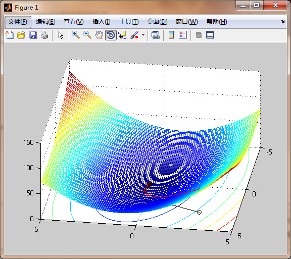
f = @(x1,x2) x1.^2 + x1.*x2 + 3*x2.^2;

m = -5:0.1:5;
[X,Y] = meshgrid(m);
Z = f(X,Y);

% plot objective function contours for visualization:
figure(1); clf; meshc(X,Y,Z); hold on

% redefine objective function syntax for use with optimization:
f2 = @(x) f(x(1),x(2));

% gradient descent algorithm:
while and(gnorm>=tol, and(niter <= maxiter, dx >= dxmin))
% calculate gradient:
g = grad(x);
gnorm = norm(g);
% take step:
xnew = x - alpha*g;
% check step
if ~isfinite(xnew)
display(['Number of iterations: ' num2str(niter)])
error('x is inf or NaN')
end
% plot current point
plot([x(1) xnew(1)],[x(2) xnew(2)],'ko-')
plot3([x(1) xnew(1)],[x(2) xnew(2)], [f(x(1),x(2)) f(xnew(1),xnew(2))]...
,'r+-');
refresh
% update termination metrics
niter = niter + 1;
dx = norm(xnew-x);
x = xnew;

end
xopt = x;
fopt = f2(xopt);
niter = niter - 1;

% define the gradient of the objective
function g = grad(x)
g = [2*x(1) + x(2)
x(1) + 6*x(2)];