机器学习初步练习题
2016-06-29 10:00
411 查看
1. 写一个函数,能将一个多类别变量转为多个二元虚拟变量,不能使用 sklearn 库。
将一个多类别变量转为多个二元虚拟变量,是数据预处理时常用的一种方法。举个例子:以性别 Sex 为例,原本一个变量,因为其取值可以是['male','female'],而将其平展开为 Sex_male 和 Sex_female 两个变量。
原本 Sex 取值为 male 的,在转换后的新变量 Sex_male 下取值为 1,在新变量 Sex_female 下取值为 0
原本 Sex 取值为 female 的,在转换后的新变量 Sex_male 下取值为 0,在新变量 Sex_female 下取值为 1
因为有些数据挖掘算法,特别是某些分类算法,要求属性是分类属性形式,发现关联模式的算法还要求数据是二元属性形式,这样就需要将连续属性转换成分类属性,即离散化,并且连续和离散属性可能都需要转换成一个或多个二元属性(二元化)。如果一个分类属性类别过多,且某些值出现不频繁,则可根据挖掘任务合并某些值以减少类别的数目。
在 Python 编程中,一般是将 DataFrame 中的一列变为多列,一列即一个 Series,转换成一个包含多 Series 即多列的 DataFrame,然后再将生成的 DataFrame 附加到原 DataFrame 上。
pandas.get_dummies 提供了这种功能。下面以性别 Sex 为例做个演示。
import pandas as pd
import numpy as np
data = {
'Name': ['Richard Dawkins', 'Eileen Chang', 'Steven Pinker', 'Madonna Ciccone', 'Herbert A. Simon'],
'Year': [1941, 1920, 1954, 1958, 1916 ],
'Sex': ['male', 'female', 'male', 'female', 'male']
}
famous_df = pd.DataFrame(data)
famous_df| Name | Sex | Year | |
|---|---|---|---|
| 0 | Richard Dawkins | male | 1941 |
| 1 | Eileen Chang | female | 1920 |
| 2 | Steven Pinker | male | 1954 |
| 3 | Madonna Ciccone | female | 1958 |
| 4 | Herbert A. Simon | male | 1916 |
print type(famous_df['Sex']) # 输入 Series
dummies_Sex = pd.get_dummies(famous_df['Sex'], prefix= 'Sex') # 对 Sex 变量二元化,prefix 为新变量的前缀,默认是原列名
print type(dummies_Sex) # 输出 DataFrame
print dummies_Sex.head()
<class 'pandas.core.series.Series'>
<class 'pandas.core.frame.DataFrame'>
Sex_female  Sex_male
0         0.0       1.0
1         1.0       0.0
2         0.0       1.0
3         1.0       0.0
4         0.0       1.0
famous_df = pd.concat([famous_df, dummies_Sex], axis=1) # 使用 concat 把生成的 DataFrame 附加到原 DataFrame 上
print famous_df
Name     Sex  Year  Sex_female  Sex_male
0   Richard Dawkins    male  1941         0.0       1.0
1      Eileen Chang  female  1920         1.0       0.0
2     Steven Pinker    male  1954         0.0       1.0
3   Madonna Ciccone  female  1958         1.0       0.0
4  Herbert A. Simon    male  1916         0.0       1.0
Sex 变量变成了两个二元变量 Sex_female 和 Sex_male。
这里我们写个自定义函数来实现跟 pandas.get_dummies 一样的功能。
函数名:OneVarToMany
参数:
data : Series,一个多类别变量
prefix : string, 新变量名前缀,默认为 None
prefix_sep : string, 如果有前缀,前缀和变量名的分隔符,默认为 '_'
many_na : bool, 是否为 NaN 值添加一列,如果为 False 则忽略 NaNs,默认为 False
返回值:
dfmany : DataFrame
def OneVarToMany(data, prefix=None, prefix_sep='_', dummy_na=False): # 二元化函数
dfmany = pd.DataFrame() # 先定义个空的 DataFrame
n = data.count() # 取得样本个数
colNames = data.unique() # 取分类变量的值作为新变量名
if(dummy_na == False):
colNames = colNames[colNames!='nan']

for i in range(colNames.shape[0]): # 遍历每个变量名,创建相应的 Series 并附加到 dfmany
colName = colNames[i]
seriesobj = pd.Series(np.zeros(n, dtype = 'int8')) # 先生成长度为 n 全为 0 的向量
seriesobj.ix[data[data == colName].index] = 1 # 修改相应的值为 1
if(prefix != None):
colName = prefix + prefix_sep + colName
seriesobj.name = colName # 修改列名
dfmany = pd.concat([dfmany, seriesobj], axis=1) # 将新生成的 Series 附加到 DataFrame 上
return dfmany
在数据集上测试下该函数。
sdata = {
'Name': ['Richard Dawkins', 'Eileen Chang', 'Steven Pinker', 'Madonna Ciccone', 'Herbert A. Simon'],
'Year': [1941, 1920, 1954, 1958, 1916 ],
'Sex': ['male', 'female', 'male', 'female', 'male']
}
df = pd.DataFrame(sdata)
dummies_Sex = OneVarToMany(df['Sex'], prefix= 'Sex')
df = pd.concat([df, dummies_Sex], axis=1)
print df
Name Sex Year Sex_male Sex_female 0 Richard Dawkins male 1941 1 0 1 Eileen Chang female 1920 0 1 2 Steven Pinker male 1954 1 0 3 Madonna Ciccone female 1958 0 1 4 Herbert A. Simon male 1916 1 0
结果跟 pandas.get_dummies 一样。
2. 写一个函数,实现交叉验证的功能,不能使用sklearn库。
交叉验证,就是把数据分为两部分,一部分用于训练,一部分用于验证。sklearn.cross_validation.train_test_split 即实现这个功能。举个例子:
import numpy as np
from sklearn.cross_validation import train_test_split

X, y = np.arange(10).reshape((5, 2)), range(5) # 生成 X 和 y
print X
print y
[[0 1]
[2 3]
[4 5]
[6 7]
[8 9]]
[0, 1, 2, 3, 4]
X_train, X_test, y_train, y_test = train_test_split(X, y, train_size=0.75, random_state=42) # test_size 指定测试集的比例
print X_train
print X_test
print y_train
print y_test
[[4 5]
[0 1]
[6 7]]
[[2 3]
[8 9]]
[2, 0, 3]
[1, 4]
下面自定义函数实现类似功能,相当于 sklearn.cross_validation.train_test_split 的简化版,输入数据类型限定为 numpy.array。
函数名:data_split
参数:
x_arrays : numpy.array,要分离的自变量数据
y_arrays : numpy.array,要分离的因变量数据
train_size : float, int(默认为 float),如果是 float,应在 0 到 1 之间,则按比例提取数据到 train 中,如果是 int,则表示训练样本个数
random_state : int 随机种子
返回值:
splitting : list, length = 2 * len(arrays),返回分离后的训练集和测试集
import random
def data_split(x_arrays, y_arrays, train_size = 0.75, random_state= 12345):
n = x_arrays.shape[0] # 取得全部样本个数
sample_count = 0

# 先排除一些输入错误的情况
if(y_arrays.shape[0] != n): # 自变量和因变量矩阵的样本个数不等
raise Exception("The length of independent variable and dependent variable are not equal.")

if(type(train_size) == int): # 计算训练集的样本个数
if(train_size > n):
raise Exception("The train_size cannot be bigger than the length of the whole datasets.")
sample_count = train_size
elif(type(train_size) == float): # 如果 train_size 是浮点数,应该在 0 和 1 之间,表示比例
if(train_size<0 or train_size>1):
raise Exception("The train_size must be between 0 and 1.")
sample_count = int(train_size*n)
else:
raise Exception("The train_size must be int or float.")

# 开始干正事儿
random.seed(random_state) # 设随机种子
listrange = range(0, n)
train_index = random.sample(listrange, sample_count) # 从 n 个样本中随机挑出 sample_count 个作为训练集
test_index = filter(lambda x : x not in train_index, listrange)
X_train = x_arrays[train_index,:] # 训练集自变量
X_test = x_arrays[test_index,:] # 测试集自变量
y_train = y_arrays[train_index] # 训练集因变量
y_test = y_arrays[test_index] # 测试集因变量

return X_train, X_test, y_train, y_test
测试一下。
X, y = np.arange(10).reshape((5, 2)), np.arange(5) # 在前面 train_test_split 的例子中 y 是 list,这里方便起见,y 为 numpy.array
X_train, X_test, y_train, y_test = data_split(X, y, train_size=0.75, random_state=42)
print X_train
print X_test
print y_train
print y_test
[[6 7]
[0 1]
[8 9]]
[[2 3]
[4 5]]
[3 0 4]
[1 2]
结果跟 sklearn.cross_validation.train_test_split 一样。
3. 使用 sklearn 库中的其他分类方法,来预测 titanic 的生存情况。
1912 年 4 月 15 日,载着 1316 号乘客和 891 名船员的豪华巨轮“泰坦尼克号”与冰山相撞而沉没,这场海难被认为是 20 世纪人间十大灾难之一。船上共 2208 名船员和乘客,但船上的救生艇仅能供 1178 人使用,最终只有 705 人生还。关于这场灾难详情,有不少记录可供查阅。以前看到一条有趣的微博,不知道是不是真的:
1898年,一个美国作家写了一篇小说,讲一艘名为 Titan 的豪华游轮,从英国出发做穿越大西洋的处女航,结果撞冰山沉没了。由于救生艇太少,死了很多人。14 年以后,Titanic的悲剧发生了。这个作家叫 Morgan Robertson,小说名为 "The Wreck of the Titan or, Futility"。小说里的 Titan 和现实中的 Titanic 在长度、吨位,客容量、推行器数量,救生艇数量等方面都惊人的相似。这个跟香港风水大师预言日本地震海啸的故事有一拼。——子夏曰
这个数据集是 1309 名乘客的资料。
数据包含的字段如下:
PassengerID
Survived(存活与否)
Pclass(客舱等级)
Name(姓名)
Sex(性别)
Age(年龄)
SibSp(亲戚和配偶在船数量)
Parch(父母孩子的在船数量)
Ticket(票编号)
Fare(价格)
Cabin(客舱位置)
Embarked(上船的港口编号)
数据读取
passenger_train = pd.read_csv('./Data/Titanic/train.csv', header=0)
passenger_test = pd.read_csv('./Data/Titanic/test.csv', header=0)
passenger_train.head()| PassengerId | Survived | Pclass | Name | Sex | Age | SibSp | Parch | Ticket | Fare | Cabin | Embarked | |
|---|---|---|---|---|---|---|---|---|---|---|---|---|
| 0 | 1 | 0 | 3 | Braund, Mr. Owen Harris | male | 22.0 | 1 | 0 | A/5 21171 | 7.2500 | NaN | S |
| 1 | 2 | 1 | 1 | Cumings, Mrs. John Bradley (Florence Briggs Th... | female | 38.0 | 1 | 0 | PC 17599 | 71.2833 | C85 | C |
| 2 | 3 | 1 | 3 | Heikkinen, Miss. Laina | female | 26.0 | 0 | 0 | STON/O2. 3101282 | 7.9250 | NaN | S |
| 3 | 4 | 1 | 1 | Futrelle, Mrs. Jacques Heath (Lily May Peel) | female | 35.0 | 1 | 0 | 113803 | 53.1000 | C123 | S |
| 4 | 5 | 0 | 3 | Allen, Mr. William Henry | male | 35.0 | 0 | 0 | 373450 | 8.0500 | NaN | S |
print passenger_train.PassengerId.count() # 看下训练集的人数
print passenger_test.PassengerId.count() # 测试集的人数
891
418
print passenger_train.Survived.value_counts()
0    549
1    342
Name: Survived, dtype: int64
训练集中一共 891 名乘客,存活的是 342 人,死亡 549 人。
先看下是不是小孩的生存率要高些。这里小孩定义为 14 岁以下。
passenger_train.info() # 查看信息
<class 'pandas.core.frame.DataFrame'>
RangeIndex: 891 entries, 0 to 890
Data columns (total 12 columns):
PassengerId    891 non-null int64
Survived       891 non-null int64
Pclass         891 non-null int64
Name           891 non-null object
Sex            891 non-null object
Age            714 non-null float64
SibSp          891 non-null int64
Parch          891 non-null int64
Ticket         891 non-null object
Fare           891 non-null float64
Cabin          204 non-null object
Embarked       889 non-null object
dtypes: float64(2), int64(5), object(5)
memory usage: 83.6+ KB
数据基本完整,只有 Age、Cabin 和 Embarked 三个字段有数据缺失。先对年龄字段做个补全。
passenger_train.ix[passenger_train['Age'].isnull(),'Age'] = passenger_train['Age'].median() # 年龄取个中间值
%matplotlib inline
import matplotlib.pyplot as plt;
fig, axes = plt.subplots(1, 3, figsize=(12, 3))
passenger_train.Survived.value_counts().sort_index().plot(kind = 'bar', ax =axes[0]); # 这里加上 sort_index() 是为了统一 index 中的次序
passenger_train[passenger_train.Age<14].Survived.value_counts().sort_index().plot(kind = 'bar', ax =axes[1]); # 小孩的死亡和生存数量对比
passenger_train[passenger_train.Age>=14].Survived.value_counts().sort_index().plot(kind = 'bar', ax =axes[2]); # 大人的死亡生存数量对比
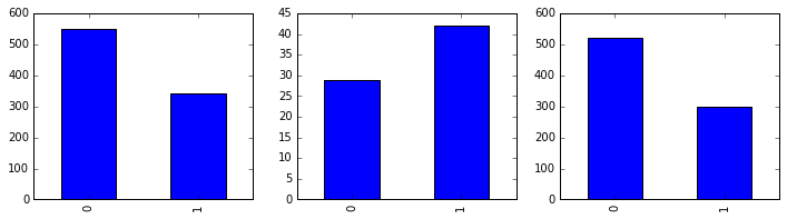
print passenger_train[passenger_train.Age<14].PassengerId.count() # 小孩数量
print passenger_train[passenger_train.Age>=14].PassengerId.count() # 大人数量
71
643
由上图可见,在整体人数生存人数比死亡人数低的情况下,小孩的生存数量比死亡数量高,大人必定死亡得更多。确实是充分照顾了小孩儿的。
再来看下性别对生存存亡的影响。
fig, axes = plt.subplots(1, 3, figsize=(12, 3))
passenger_train.Survived.value_counts().sort_index().plot(kind = 'bar', ax =axes[0], title='All');
passenger_train[passenger_train.Sex=='female'].Survived.value_counts().sort_index().plot(kind = 'bar', ax =axes[1], title='female');
passenger_train[passenger_train.Sex=='male'].Survived.value_counts().sort_index().plot(kind = 'bar', ax =axes[2], title='male');
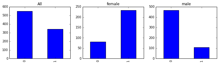
print passenger_train[passenger_train.Sex=='female'].PassengerId.count() # 女性数量
print passenger_train[passenger_train.Sex=='male'].PassengerId.count() # 男性数量
314
577
上面的结果让人动容,女性的生存人数远远大于死亡人数,男性的死亡人数远远大于生存人数。从上面的柱状图对比,可以想象男性在这场灾难中展现出的让人敬重的绅士风度。
再来看下客舱等级对存亡的影响。
泰坦尼克号的奢华和精致堪称空前。船上配有室内游泳池、健身房、土耳其浴室、图书馆、电梯和壁球室。头等舱的公共休息室由精细的木质镶板装饰,配有高级家具以及其他各种高级装饰,并竭尽全力提供了以前从未见过的服务水平。阳光充裕的巴黎咖啡馆为头等舱乘客提供各种高级点心。泰坦尼克号的二等舱甚至是三等舱的居住环境和休息室都同样高档,甚至可以和当时许多客轮的头等舱相比。三台电梯专门为头等舱乘客服务;作为革新,二等舱乘客也有一台电梯使用,不过,三等舱的乘客仍然需要爬楼梯。
passenger_train.Pclass.value_counts()
3    491
1    216
2    184
Name: Pclass, dtype: int64
fig, axes = plt.subplots(1, 4, figsize=(12, 3))
passenger_train.Survived.value_counts().sort_index().plot(kind = 'bar', ax =axes[0], title='All Class');
passenger_train[passenger_train.Pclass==1].Survived.value_counts().sort_index().plot(kind = 'bar', ax =axes[1], title='Class 1');
passenger_train[passenger_train.Pclass==2].Survived.value_counts().sort_index().plot(kind = 'bar', ax =axes[2], title='Class 2');
passenger_train[passenger_train.Pclass==3].Survived.value_counts().sort_index().plot(kind = 'bar', ax =axes[3], title='Class 3');
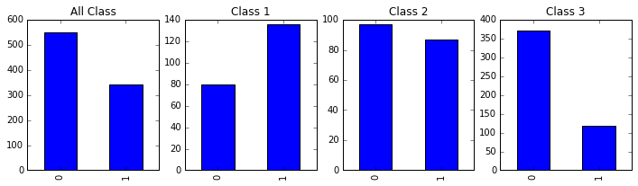
从上图明显看出,一等舱的生存率最高,二等舱次之,三等舱最低。可见客舱等级确实影响了乘客的生存几率。
我们再来看下,不同等级客舱的小孩儿的生存几率有没有差别。
fig, axes = plt.subplots(1, 4, figsize=(12, 3))
passenger_train[passenger_train.Age<14].Survived.value_counts().sort_index().plot(kind = 'bar', ax =axes[0], title='All Children');
passenger_train[(passenger_train.Pclass==1) & (passenger_train.Age<14)]    \
.Survived.value_counts().sort_index().plot(kind = 'bar', ax =axes[1], title='Class 1 Children'); # 头等舱小孩
passenger_train[(passenger_train.Pclass==2) & (passenger_train.Age<14)]    \
.Survived.value_counts().sort_index().plot(kind = 'bar', ax =axes[2], title='Class 2 Children'); # 二等舱小孩
passenger_train[(passenger_train.Pclass==3) & (passenger_train.Age<14)]    \
.Survived.value_counts().sort_index().plot(kind = 'bar', ax =axes[3], title='Class 3 Children'); # 三等舱小孩
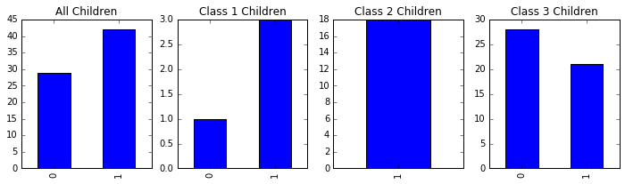
print passenger_train[passenger_train.Age<14].PassengerId.count() # 所有小孩
print passenger_train[(passenger_train.Age<14) & (passenger_train.Survived==0)].PassengerId.count() # 死亡
print passenger_train[(passenger_train.Age<14) & (passenger_train.Survived==1)].PassengerId.count() # 存活
print passenger_train[(passenger_train.Age<14) & (passenger_train.Survived==0) & (passenger_train.Pclass==3)].PassengerId.count() # 死亡
print passenger_train[(passenger_train.Age<14) & (passenger_train.Survived==1) & (passenger_train.Pclass==3)].PassengerId.count() # 存活
71
29
42
28
21
一共 71 个 14 岁以下的小孩儿,死亡 29 个,存活 42 个。其中头等舱一共 4 个小孩,死亡 1 个,存活 3 个;二等舱 18 个小孩全部存活;三等舱 49 个小孩,死亡 28 个,存活 21 个。从柱状图上也可以看出,上等客舱的小孩儿存活率更高。
再来比较头等舱的男人和三等舱的小孩儿的存活个数。
fig, axes = plt.subplots(1, 2, figsize=(12, 3))
passenger_train[(passenger_train.Pclass==1) & (passenger_train.Age>=14) & (passenger_train.Sex=='male')]    \
.Survived.value_counts().sort_index().plot(kind = 'bar', ax =axes[0], title='Class 1 Men'); # 头等舱男人
passenger_train[(passenger_train.Pclass==3) & (passenger_train.Age<14)]    \
.Survived.value_counts().sort_index().plot(kind = 'bar', ax =axes[1], title='Class 3 Children'); # 三等舱小孩
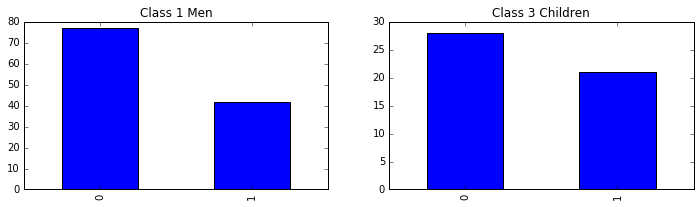
目测三等舱小孩儿的存活几率要高些。
既然到这了,我们就索性再看下头等舱的男人和三等舱的妇女的存活个数。
fig, axes = plt.subplots(1, 2, figsize=(12, 3))
passenger_train[(passenger_train.Pclass==1) & (passenger_train.Age>=14) & (passenger_train.Sex=='male')]    \
.Survived.value_counts().sort_index().plot(kind = 'bar', ax =axes[0], title='Class 1 Men'); # 头等舱男人
passenger_train[(passenger_train.Pclass==3) & (passenger_train.Age>=14) & (passenger_train.Sex=='female')]    \
.Survived.value_counts().sort_index().plot(kind = 'bar', ax =axes[1], title='Class 3 Women'); # 三等舱妇女
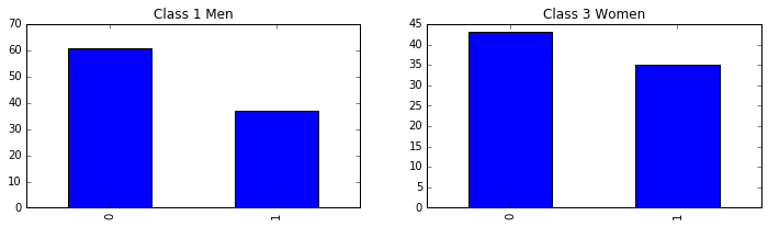
头等舱男人不比三等舱妇女存活几率高,女士比等级优先。
目前我们看了性别、年龄和等级对存亡的影响,这三个因素的影响都是很明显的。再来看下 SibSp(亲戚和配偶在船数量)、Parch(父母孩子的在船数量)对存亡的影响。
fig, axes = plt.subplots(1, 3, figsize=(12, 3))
passenger_train.Survived.value_counts().sort_index().plot(kind = 'bar', ax =axes[0], title='All');
passenger_train[(passenger_train.SibSp>0)]    \
.Survived.value_counts().sort_index().plot(kind = 'bar', ax =axes[1], title='SibSp'); # 亲戚和配偶在船数量
passenger_train[passenger_train.Parch>0]    \
.Survived.value_counts().sort_index().plot(kind = 'bar', ax =axes[2], title='Parch'); # 父母孩子的在船数量
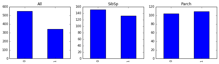
从上图看,有亲戚和配偶,或者有父母孩子在船,存活率是要高些。
再来看下 Embarked(上船的港口编号)。
passenger_train.Embarked.value_counts()
S    644
C    168
Q     77
Name: Embarked, dtype: int64
fig, axes = plt.subplots(1, 4, figsize=(12, 3))
passenger_train.Survived.value_counts().sort_index().plot(kind = 'bar', ax =axes[0], title='All');
passenger_train[passenger_train.Embarked == 'S']    \
.Survived.value_counts().sort_index().plot(kind = 'bar', ax =axes[1], title='S'); # S
passenger_train[passenger_train.Embarked == 'C']    \
.Survived.value_counts().sort_index().plot(kind = 'bar', ax =axes[2], title='C'); # C
passenger_train[passenger_train.Embarked == 'Q']    \
.Survived.value_counts().sort_index().plot(kind = 'bar', ax =axes[3], title='Q'); # Q

上面港口编号为 C 的人存活比例比其它要高,但我认为这只是一个很随机的结果,随机不等于均匀,不是存活的原因。如果这也能算,那要从船上找到此类原因就多了去了。
再来看下票价 Fare,统计下各等级船舱的票价频次。
fig, axes = plt.subplots(3, 1, figsize=(12, 6))
passenger_train.Fare.hist(bins = 100, ax=axes[0])
passenger_train[passenger_train.Pclass==1].Fare.hist(bins = 100, ax=axes[0]); # 一等舱票价频次
passenger_train[passenger_train.Pclass==2].Fare.hist(bins = 100, ax=axes[1]); # 二等舱票价频次
passenger_train[passenger_train.Pclass==3].Fare.hist(bins = 100, ax=axes[2]); # 三等舱票价频次
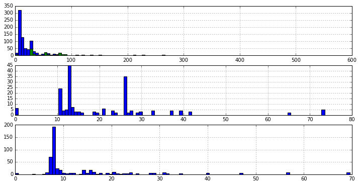
船舱等级越高,票价越高,票价 Fare 跟客舱等级是同一性质的属性,客舱等级已经是个非常好的价格离散化后的结果了。所以,这里的预测就不要 Fare 属性了。
客舱位置 Cabin 缺失值太多,去除;Ticket 值太多,没意义,去除;Name 无意义,去除。
去除无关属性数据
passenger_train = passenger_train.drop('Name', axis=1)
passenger_train = passenger_train.drop('Ticket', axis=1)
passenger_train = passenger_train.drop('Embarked', axis=1)
passenger_train = passenger_train.drop('Cabin', axis=1)
passenger_train = passenger_train.drop('Fare', axis=1)
passenger_train = passenger_train.drop('PassengerId', axis=1)
passenger_train.head()
| Survived | Pclass | Sex | Age | SibSp | Parch | |
|---|---|---|---|---|---|---|
| 0 | 0 | 3 | male | 22.0 | 1 | 0 |
| 1 | 1 | 1 | female | 38.0 | 1 | 0 |
| 2 | 1 | 3 | female | 26.0 | 0 | 0 |
| 3 | 1 | 1 | female | 35.0 | 1 | 0 |
| 4 | 0 | 3 | male | 35.0 | 0 | 0 |
passenger_train.Sex = passenger_train.Sex.map({"male": 1, "female": 0}) # 做个映射passenger_train.ix[passenger_train.Age<15,'Age'] = 0 passenger_train.ix[(passenger_train.Age>=15) & (passenger_train.Age<30),'Age'] = 1 passenger_train.ix[(passenger_train.Age>=30) & (passenger_train.Age<45),'Age'] = 2 passenger_train.ix[(passenger_train.Age>=45) & (passenger_train.Age<60),'Age'] = 3 passenger_train.ix[passenger_train.Age>=60,'Age'] = 4
passenger_train.head()
| Survived | Pclass | Sex | Age | SibSp | Parch | |
|---|---|---|---|---|---|---|
| 0 | 0 | 3 | 1 | 1.0 | 1 | 0 |
| 1 | 1 | 1 | 0 | 2.0 | 1 | 0 |
| 2 | 1 | 3 | 0 | 1.0 | 0 | 0 |
| 3 | 1 | 1 | 0 | 2.0 | 1 | 0 |
| 4 | 0 | 3 | 1 | 2.0 | 0 | 0 |
passenger_train.info() # 查看信息
<class 'pandas.core.frame.DataFrame'>
RangeIndex: 891 entries, 0 to 890
Data columns (total 6 columns):
Survived    891 non-null int64
Pclass      891 non-null int64
Sex         891 non-null int64
Age         891 non-null float64
SibSp       891 non-null int64
Parch       891 non-null int64
dtypes: float64(1), int64(5)
memory usage: 41.8 KB
对年龄字段做个处理。
from sklearn.cross_validation import train_test_split
X_train, X_test, y_train, y_test = train_test_split(passenger_train.drop('Survived', axis=1), passenger_train.Survived, train_size=0.8)下面尝试各种分类算法。
from sklearn import datasets
from sklearn import cross_validation
from sklearn import linear_model
from sklearn import metrics
from sklearn import tree
from sklearn import neighbors
from sklearn import svm
from sklearn import ensemble
from sklearn import cluster
先试下 Logistic 回归。
classifier = linear_model.LogisticRegression()
classifier.fit(X_train, y_train)
LogisticRegression(C=1.0, class_weight=None, dual=False, fit_intercept=True,
intercept_scaling=1, max_iter=100, multi_class='ovr', n_jobs=1,
penalty='l2', random_state=None, solver='liblinear', tol=0.0001,
verbose=0, warm_start=False)
y_test_pred = classifier.predict(X_test)
print(metrics.classification_report(y_test, y_test_pred)) # 真实的 y 和预测的 y
precision    recall  f1-score   support

0       0.84      0.87      0.85       112
1       0.77      0.73      0.75        67

avg / total       0.81      0.82      0.81       179
precision 是精准度,recall 是召回率,fs-score 是 F1 值。各个指标还算不错。再来看混淆矩阵。
metrics.confusion_matrix(y_test, y_test_pred)
array([[97, 15],
[18, 49]])
预测正确的有 146 人,错误 33 人。效果还不错。
再来尝试其它分类方法。决策树:
classifier = tree.DecisionTreeClassifier() # 决策树
classifier.fit(X_train, y_train)
y_test_pred = classifier.predict(X_test)
metrics.confusion_matrix(y_test, y_test_pred)
array([[101,  13],
[ 18,  47]])
classifier = neighbors.KNeighborsClassifier() # K 近邻
classifier.fit(X_train, y_train)
y_test_pred = classifier.predict(X_test)
metrics.confusion_matrix(y_test, y_test_pred)
array([[97, 17],
[15, 50]])
classifier = svm.SVC() # 支持向量机
classifier.fit(X_train, y_train)
y_test_pred = classifier.predict(X_test)
metrics.confusion_matrix(y_test, y_test_pred)
array([[101,  13],
[ 15,  50]])
classifier = ensemble.RandomForestClassifier() # 随机森林
classifier.fit(X_train, y_train)
y_test_pred = classifier.predict(X_test)
metrics.confusion_matrix(y_test, y_test_pred)
array([[101,  13],
[ 18,  47]])
从以上各种分类算法的混淆矩阵来看,支持向量机的预测效果是最好的,只预测错了 28 个人。
4. 研究 kaggle 中的 Digit Recognizer 数据,尝试用一些特征工程来提取数字的特征,并放入分类器中观察预测准确率,相对直接使用原始变量是否有提升。
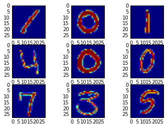
train.csv 和 test.csv 包含 1~9 的手写数字的灰度图片。每幅图片都是 28 个像素的高度和宽度,共 28*28=784 个像素点,每个像素值都在 0~255 之间。train.csv 包含 785 列,因为第 1 列是手写数字的真实值,后面的 784 列都是像素值。除第一行外,有 42000 条数据。
test.csv 除了不包含 label 列,其它跟 train.csv 一样。除第一行外,有 28000 条数据。
先来看看 train.csv 里的灰度图片是什么样子。
digitTrain = pd.read_csv('./Data/Digit-Recognizer/train.csv')img = digitTrain.values[0:11,1:] fig = plt.figure() for i in range(0,9,1): print "\ncurrent num is: %d" % i px = img[i,:] pix = [] for j in range(28): pix.append([]) for k in range(28): pix[j].append(px[j*28+k]) ax = fig.add_subplot(330+i+1) ax.imshow(pix) plt.show()
current num is: 0

current num is: 1

current num is: 2

current num is: 3

current num is: 4

current num is: 5

current num is: 6

current num is: 7

current num is: 8
首先将每个图片的像素值都变成二进制形式,像素值大于 0 的变成 1。
digitdata = digitTrain.ix[:,1:] # 像素数据
digitdata = digitdata.replace([1,255], 1)
digittest = digitTrain.ix[:,0] # Label 数据
X_train, X_test, y_train, y_test = cross_validation.train_test_split(digitdata, digittest, train_size=0.7) # 70% 用于训练,30% 用于检验
经过分析,该数据集适合用 K 最近邻算法。
classifier = neighbors.KNeighborsClassifier() # K 近邻
classifier.fit(X_train, y_train)
y_test_pred = classifier.predict(X_test)
metrics.confusion_matrix(y_test, y_test_pred)
array([[1220,    5,    1,    0,    1,    1,    1,    0,    0,    1],
[   1, 1385,    3,    1,    1,    0,    1,    2,    0,    1],
[  31,   39, 1156,    5,    1,    0,    2,   23,    1,    2],
[  20,   57,    9, 1153,    0,   11,    1,    8,    6,    3],
[  27,   46,    4,    0, 1118,    0,    4,    1,    0,   30],
[  31,   30,    1,   20,    0, 1007,    7,    1,    0,    8],
[  42,   23,    0,    0,    1,    1, 1216,    0,    0,    0],
[  26,   46,    6,    0,    4,    0,    0, 1232,    0,    7],
[  24,   61,    7,   18,    6,   25,    7,    3, 1052,   13],
[  22,   40,    4,    8,   10,    5,    2,   27,    1, 1174]])
从混淆矩阵来看,预测结果还算不错。

相关文章推荐
- js实现仿windows文件按名称排序
- RIO-SEIO水泵流量表
- Angular新手容易碰到的坑,随时更新,欢迎订阅
- 正则表达式 ━━ 入门
- AngularJS过滤器(Filters)
- $ctags -R --fields=+iaS --extra=+q *
- UCS-2编码与UTF-8编码
- hibernate进阶之路之多对多映射(五)
- 如何获取drawable目录下的图片绝对路径
- Oracle忽略hint的几种情形
- 太用力的人跑不远
- 防止恶意频繁发送短信验证码
- Java中可变长参数的使用及注意事项
- hdu 1166
- 多源最短路(codevs 1077)
- 专题四-1006-典型Kruskal算法应用
- springmvc和spring的父子容器关系
- ubuntu 14.04使用apt-get安装最新稳定版nginx的方法
- 必做: 1041、1024、1077、2218、1183(较难)
- hdu 1166