机器学习学习笔记 PRML Chapter 1.5 : Decision Theory

Chapter 1.5 : Decision Theory

PRML, OXford University Deep Learning Course, Machine Learning, Pattern Recognition

Christopher M. Bishop, PRML, Chapter 1 Introdcution

1. PRML所需要的三论:

Probability theory: provides us with a consistent mathematical framework for quantifying and manipulating uncertainty.

Decision theory: allows us to make optimal decisions in situations involving uncertainty such as those encountered in pattern recognition.

Information theory:

Inference step & Decision step

- The joint probability distribution p(x,t) provides a complete summary of the uncertainty associated with these variables. Determination of p(x,t) from a set of training data is an example of inference and is typically a very difficult problem whose solution forms the subject of much of this book.

- In a practical application, however, we must often make a specific prediction for the value of t, or more generally take a specific action based on our understanding of the values t is likely to take, and this aspect is the subject of decision theory.

2. An example

Problem Description:

Consider, for example, a medical diagnosis problem in which we have taken an X-ray image of a patient, and we wish to determine whether the patient has cancer or not.

Representation: choose t to be a binary variable such that t=0 corresponds to class C1 and t=1 corresponds to class C2.

Inference Step: The general inference problem then involves determining the joint distribution p(x,Ck), or equivalently p(x,t), which gives us the most complete probabilistic description of the situation.

Decision Step: In the end we must decide either to give treatment to the patient or not, and we would like this choice to be optimal in some appropriate sense. This is the decision step, and it is the subject of decision theory to tell us how to make optimal decisions given the appropriate probabilities.

How to predict?

Using Bayes’ theorem, these probabilities can be expressed in the form

Posteriorp(Ck∣x)=Likelihood⋅PriorEvidence⟺=p(x∣Ck)p(Ck)p(x)=p(x∣Ck)p(Ck)∑2j=1p(x∣Cj)p(Cj)=p(x∣Ck)p(Ck)p(x∣C1)p(C1)+p(x∣C2)p(C2)

If our aim is to minimize the chance of assigning x to the wrong class Ck,k=1,2, then intuitively we would choose the class having the higher posterior probability. We now show that this intuition is correct, and we also discuss more general criteria for making decisions.

Our objectives vary among those:

- Minimizing the misclassification rate;

- Minimizing the expected loss;

补充：Criteria for making decisions【Ref -1】

1) Minimizing the misclassification rate.

2) minimizing the expected loss: 两类错误的后果可能是不同的,例如“把癌症诊断为无癌症”的后果比“把无癌症诊断为癌症”的后果更严重,又如“把正常邮件诊断为垃圾邮件”的后果比“把垃圾邮件诊断为正常邮件”的后果更严重;这时候,少犯前一错误比少犯后一错误更有意义。为此需要 loss function 对不同的错误的代价做量化。

设集合 A={a1,...,ap}是所有可能的决策，决策函α:X↦A把每个观察数据x∈X映射到一个决α(x)，则有

α(x)=argminai∈A(ai∣x)

其中 R(ai∣x) 表示条件风险:

R(ai∣x)=∑j=1cλ(ai∣ωj)P(ωj∣x)

- λ(ai∣ωj) 是对于特定的真实类别是 ωj的数据，决策为 ai 时的 loss 或 risk，即表示 λ(ai∣x∈ωj);

- P(ωj∣x) 是当观察到 x 后，类别 ωj 的后验概率。决策函数 α(x) 总是把观测数据映射到条件风险最小的决策上。

- 于是，决策函数α(x) 的总的 risk 是: R[α]=∫R(α(x)∣x)p(x)dx 即总的risk是条件风险 R(α(x)∣x) 在所有可能观测数据(特征空间)分布下的期望值。

3. Minimizing the misclassification rate

3.1 Decision Regions & Boundaries

Suppose that our goal is simply to make as few misclassifications as possible.

- Decision regions: to divide the input space into regions Rk called decision regions, one for each class, such that all points in Rk are assigned to class Ck;

- Decision boundaries or decision surfaces: The boundaries between decision regions.

3.2 Two Classes:

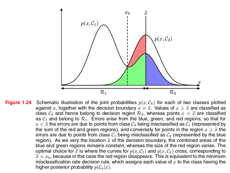
Consider the cancer problem for instance. A mistake occurs when an input vector belonging to class C1 is assigned to class C2 or vice versa. The probability of this occurring is given by

argmaxDecisonBoundariesp(mistake)=p(x∈R1,C2)+p(x∈R2,C1)=∫R1p(x,C2)dx+∫R2p(x,C1)dx⟺∫R1p(C2∣x)p(x)dx+∫R2p(C1∣x)p(x)dx (due to the common term p(x))⟺∫R1p(C2∣x)dx+∫R2p(C1∣x)dx (1.78)

Clearly to minimize p(mistake) we should arrange that each x is assigned to whichever class has the smaller value of the integrand in (1.78). This result is illustrated for two classes, and a single input variable x, in Figure 1.24.

3.3 K Classes:

For the more general case of K classes, it is slightly easier to maximize the probability of being correct, which is given by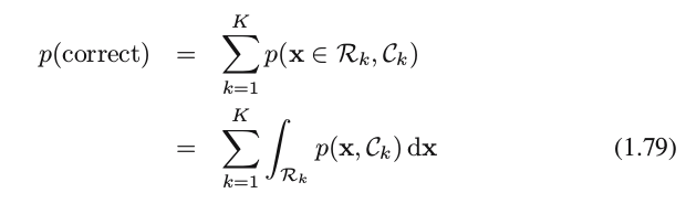



which is maximized when the regions Rk are chosen such that each x is assigned to the class for which the joint probability p(x,Ck) or equivalently posterior probability p(ck∣x) is largest.

4. Minimizing the expected loss

4.1 Problem Description:

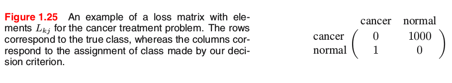
For many applications, our objective will be more complex than simply minimizing the number of misclassifications. Let us consider again the medical diagnosis problem. We note that, if a patient who does not have cancer is incorrectly diagnosed as having cancer, the consequences may be some patient distress plus the need for further investigations. Conversely, if a patient with cancer is diagnosed as healthy, the result may be premature death due to lack of treatment. Thus the consequences of these two types of mistake can be dramatically different. It would clearly be better to make fewer mistakes of the second kind, even if this was at the expense of making more mistakes of the first kind.

4.2 How to solve the problem? Introduce loss/cost function

loss function or cost function: a single, overall measure of loss incurred in taking any of the available decisions or actions, whose value they aim to minimize.

utility function: whose value they aim to maximize.

The optimal solution is the one which minimizes the loss function, or equivalently maximizes the utility function.

loss matrix:

4.3 Optimal Solution

The optimal solution is the one which minimizes the loss function. * ??? However, the loss function depends on the true class, which is unknown. * For a given input vector x, our uncertainty in the true class is expressed through the [b]joint probability distribution p(x,Ck) and so we seek instead to minimize the average loss, where the average is computed with respect to this distribution, which is given by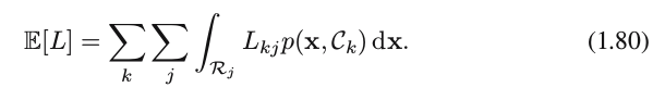



Equivalently, for each x we should minimize ∑kLkjp(x,Ck)−→−−−−p(x)common∑kLkjp(Ck∣x) to choose the corresponding optimal region Rj.

Thus the decision rule that minimizes the expected loss (1.80) is the one that assigns each new x to the class j for which the quantity



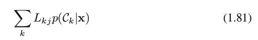
is a minimum. This is clearly trivial to do, once we know the posterior class probabilities p(Ck∣x).

5. The reject option

We have seen that classification errors arise from the regions of input space where the largest of the posterior probabilities p(Ck∣x) is significantly less than unity(i.e., the state of being in full agreement), or equivalently where the joint distributions p(x,Ck) have comparable values. These are the regions where we are relatively uncertain about class membership.

- Reject option: In some applications, it will be appropriate to avoid making decisions on the difficult cases in anticipation of a lower error rate on those examples for which a classification decision is made. This is known as the reject option. For example, in our hypothetical medical illustration, it may be appropriate to use an automatic system to classify those X-ray images for which there is little doubt as to the correct class, while leaving a human expert to classify the more ambiguous cases.

- We can achieve this by introducing a threshold θ and rejecting those inputs x for which the largest of the posterior probabilities p(Ck∣x) is less than or equal to θ. This is illustrated for the case of two classes, and a single continuous input variable x, in Figure 1.26.



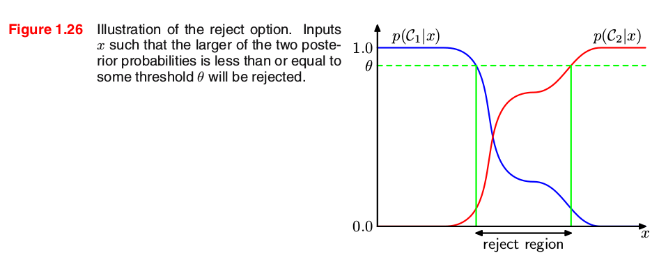
Note that setting θ=1 will ensure that all examples are rejected, whereas if there are K classes then setting θ<1/K will ensure that no examples are rejected. Thus the fraction of examples that get rejected is controlled by θ. We can easily extend the reject criterion to minimize the expected loss, when a loss matrix is given, taking account of the loss incurred when a reject decision is made.

6. Three distinct approaches to solving decision problems

The three distinct approaches are given, in decreasing order of complexity, by:

- generative models: using Bayes’ theorem to find the posterior class probabilities p(Ck∣x).

- discriminative models: to model the posterior probabilities directly.

- discriminant functions: function f(x):x↦Ck.

6.1 Generative Models

1-1) Likelihood: First solve the inference problem of determining the class-conditional densities p(x∣Ck) for each class Ck individually.

1-2) Prior: separately infer the prior class probabilities p(Ck).

1-3) Posterior: use Bayes’ theorem to find the posterior class probabilities p(Ck∣x) in the form



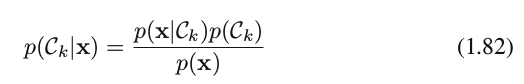
where the denominator is obtained by



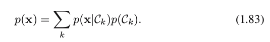
2) Equivalently, we can model the joint distribution p(x,Ck) directly and then normalize to obtain the posterior probabilities.

3) Decision Stage: use decision theory to determine class membership for each new input x.

Why called generative models?

Approaches that explicitly or implicitly model the distribution of inputs as well as outputs are known as generative models, because by sampling from them it is possible to generate synthetic data points in the input space.

Pros and Cons:

(-) Generative models is the most demanding because it involves finding the joint distribution over both x and Ck. For many applications, x will have high dimensionality, and consequently we may need a large training set in order to be able to determine the class-conditional densities to reasonable accuracy.

(+) it allows the marginal density of data p(x) to be determined from (1.83). This can be useful for outlier detection or novelty detection.

6.2 Discriminative Models:

First solve the inference problem of determining the posterior class probabilities p(Ck∣x),

and then subsequently use decision theory to assign each new x to one of the classes.

Approaches that model the posterior probabilities directly are called discriminative models.

The classification problem is usually broken down into two separate stages as do (6.1) and (6.2):

- inference stage: to use training data to learn a model for p(Ck∣x).

- decision stage: to use these posterior probabilities to make optimal class assignments.

However (6.3) provides us with a different approach, which combines the inference and decision stages into a single learning problem.

6.3 Discriminant Functions:

Discriminant functions solve both inference problem and decision problem together and simply learn a function that maps inputs x directly into decisions.

因此discriminant function 把 inference 和 decision 合为一步解决了[Ref-1]。

Disadvantage: we no longer have access to the posterior probabilities p(Ck∣x).

6.4 The Relative Merits of These Three Alternatives [Ref-1]

Generative Model 的缺点: 如果只是make classification decision, 计算 joint distribution p(x,Ck) is wasteful of computational resources, and is excessively demanding of data。一般有后验概率, 即Discriminative Models就足够了。

Discriminant function的缺点: 该方法不求后验概率posterior, but there are many powerful reasons for wanting to compute the posterior probabilities:

(1) Minimizing risk: 当 loss matrix 可能随时间改变时 (例如 financial application),如果已经有了计算出来的后验概率, 那么解决 the minimum risk decision problem 只需要适当修改(1.81)即可; 但是对于没有后验概率的discriminant function来时，只能全部从头再learning一次。

(2) Compensating for class priors: 当正负样本不平衡时(例如 X-ray 图诊断癌症, 由于cancer is rare, therefore 99.9%可能都是无癌症样本),为了获得好的分类器,需要人工做出一个balanced data set 用于training; 训练得到一个后验概率P(Ck∣x) 后，需要 compensate for the effects of the modification to the training data, 即把 P(Ck∣x) obtained from our artificially balanced data set, 除以 balanced data set 的先验P(Ck) , 再乘以真实数据(i.e., in the population)的先验 P(Ck), 从而得到了真实数据的后验概率P(Ck∣x)。没有后验概率的 discriminant function 是无法用以上方法应对正负样本不平衡问题的。

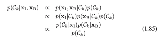
(3) Combining models(模型融合): 对于复杂应用,一个problem 被分解成a number of smaller subproblems each of which can be tackled by a separate module, 例如疾病诊断,可能除了 X-ray 图片数据xI ,还有血液检查数据 xB 。与其把这些 heterogeneous information 合在一起作为input, 更有效的方法是build one system to interpret the X-ray images and a different one to interpret the blood data。即有: to assume conditional independence based on the class Ckin the form ( the naive Bayes model)



The posterior probability, given both the X-ray and blood data, is then given by

7. Loss functions for regression

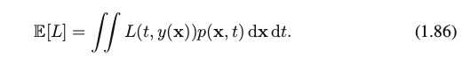
So far, we have discussed decision theory in the context of classification problems. We now turn to the case of regression problems, such as the curve fitting example discussed earlier.

Decision stage for regression: The decision stage consists of choosing a specific estimate y(x) of the value of t for each input x. Suppose that in doing so, we incur a loss L(t,y(x)). The average, or expected, loss is then given by



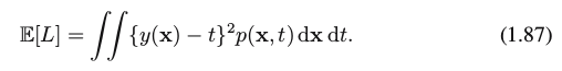
the squared loss: L(t,y(x))={(y(x)−t}2, which is substituted into (1.86), to generate the following



Solution: assume a complete flexible function y(x), we can do this formally using the calculus of variations to give


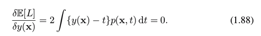
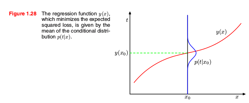
Solving for y(x), and using the sum and product rules of probability, we obtain



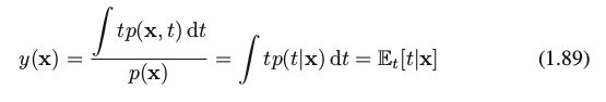
which is the conditional average of t conditioned on x and is known as the regression function. This result is illustrated in Figure 1.28.



we can identify three distinct approaches to solving regression problems given, in order of decreasing complexity, by:

(a) First solve the inference problem of determining the joint density p(x,t). Then normalize to find the conditional density p(t∣x), and finally marginalize to find the conditional mean given by (1.89).

(b) First solve the inference problem of determining the conditional density p(t∣x), and then subsequently marginalize to find the conditional mean given by (1.89).

(c) Find a regression function y(x) directly from the training data.

The relative merits of these three approaches follow the same lines as for classification problems above.

Minkowski loss: one simple generalization of the squared loss, called the Minkowski loss, whose expectation is



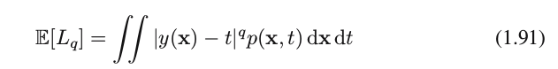
which reduces to the expected squared loss for q=2.

[1] Page 6 of PRML notes;

[2] Page 7-8 of PRML notes;