维数灾难与自编码器The Curse of Dimensionality and the Autoencoder
2016-04-04 12:58
417 查看
Let's say you're working on a cool image processing project, and your goal is to build an algorithm that analyzes faces for emotions. It takes in a 256 pixel by 256 pixel grayscale image
as its input and spits out an emotion as an answer. For example, if you passed in the following image, you'd expect the algorithm to label it as "happy."

A greyscale input image of a happy man
Now this is all well and good, but before we're satisfied with this approach, let's take a step back and think about what this really means. A 256 by 256 grayscale image corresponds to
an input vector of over 65,000 dimensions! In other words, we're trying to solve a problem in a 65,000-dimensional space. That's not a particularly easy thing to do, even for a computer! Not only are large inputs annoying to store, move around, and compute
with, but they also give rise to some pretty serious tractability concerns.
C.J. Stone in 1982, the time it takes to fit a model (specifically a nonparametric regression) to your data is at best proportional to m−p/(2p+d)m−p/(2p+d),
where mm is
the number of data points, dd is
the dimensionality of the data, and pp is
a parameter that depends on the model we are using (specifically, we are assuming that the regression function is pp times
differentiable). In a nutshell, this relation implies that we need exponentially more training examples was we increase the dimensionality of our inputs.
We can observe this graphically by considering a simple example, borrowed from Gutierrez-Osuna. Our learning algorithm divides the feature space uniformly into bins and plot all of our
training examples. We then assign each bin a label based on the predominant class that's found in that bin. Finally, for each new example that we want to classify, we just need to figure out the bin the example falls into and the label associated with that
bin!
In our toy problem, we begin by choosing a single feature (one-dimensional inputs) and divide the space into 3 simple bins:

A simple example involving one-dimensional inputs
Understandably, we notice there's too much overlap between classes, so we decide to add another feature to improve separability. But we notice that if we keep the same number of samples,
we get a 2D scatter plot that's really sparse, and it's really hard to ascertain any meaningful relationships without increasing the number of samples. If we move onto 3-dimensional inputs, it becomes even worse. Now we're trying to fill even more 33=2733=27 bins
with the same number of examples. The scatter plot is nearly empty!
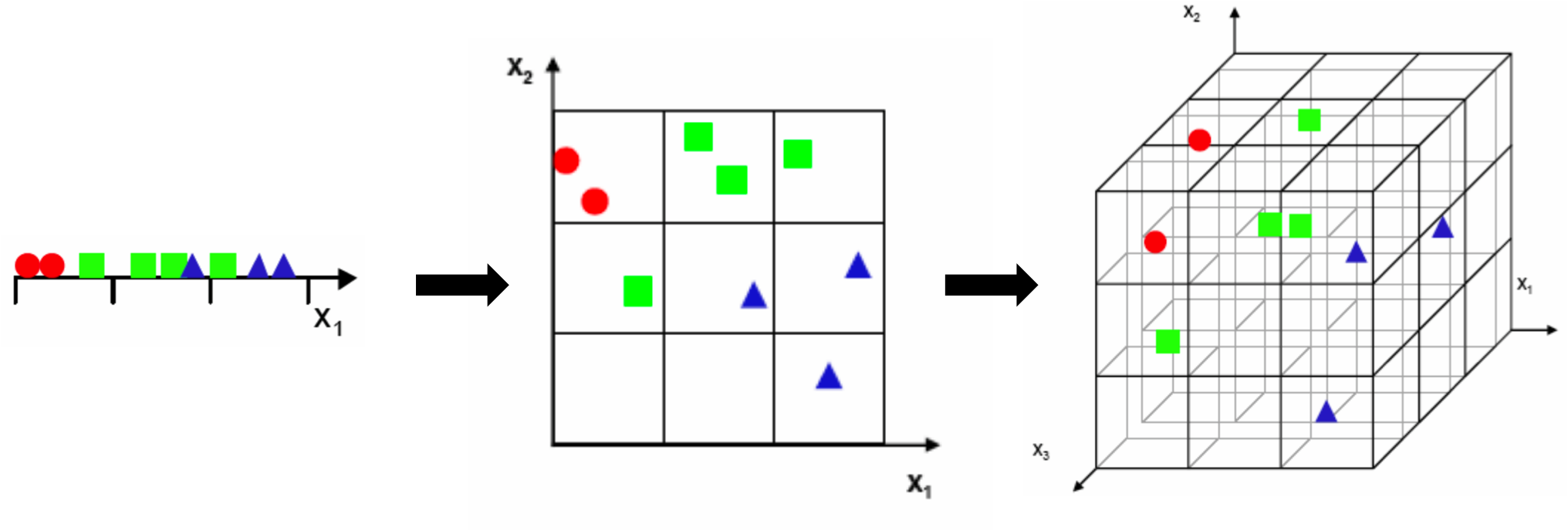
Sparsity becomes exponentially worse as dimension increases
Of important note is that this is NOT an issue that can be easily solved by more effective computing or improved hardware! For many machine learning tasks, collecting training examples
is the most time consuming part, so this mathematical result forces us to be careful about the dimensions we choose to analyze. If we are able to express our inputs in few enough dimensions, we might be able to turn an unfeasible problem into a feasible one!
our brain automatically uses to detect emotion quickly. For example, the curve of the person's lips, the extent his brow is furrowed, and the shape of his eyes all help us determine that the man in the picture is feeling happy. It turns out that these features
can be conveniently summarized by looking at the relative positioning of various facial keypoints, and the distances between them.
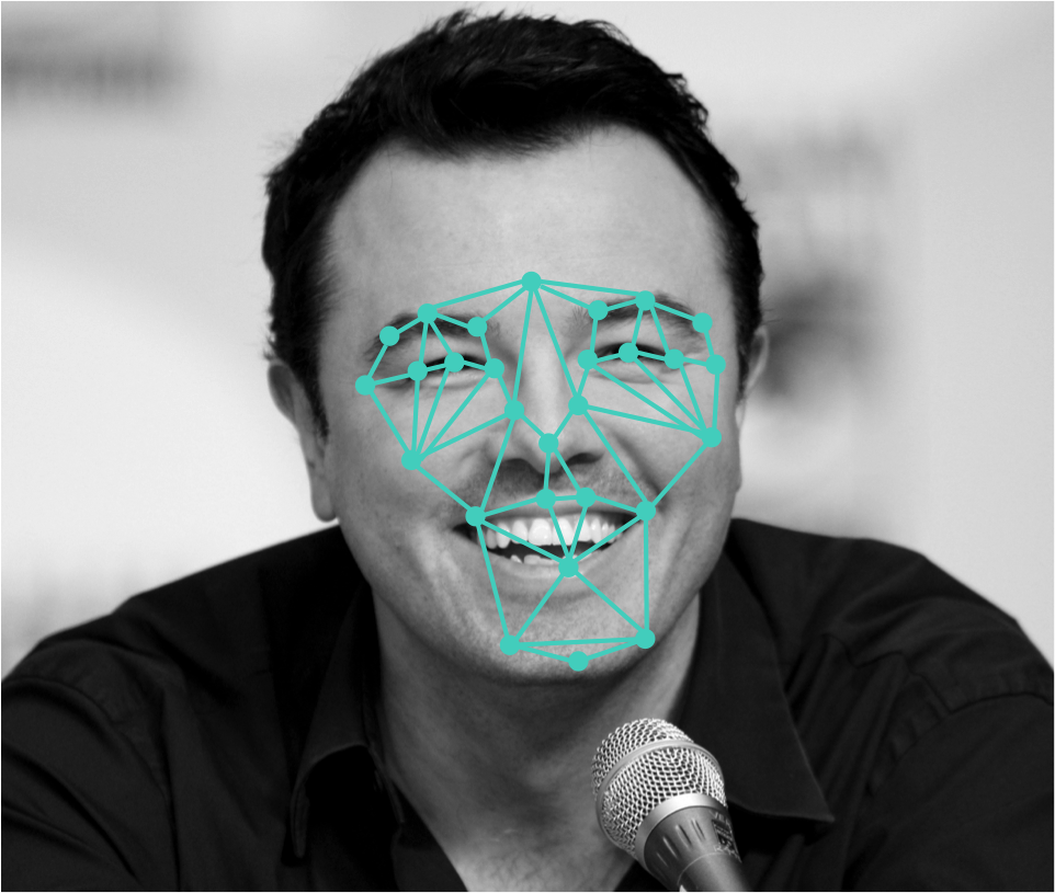
The key features of human facial expression
Obviously, this allows us to significantly reduce the dimensionality of our input (from 65,000 to about 60), but there are some limitations! Hand selection of features can take years and
years of research to optimize. For many problems, the features that matter are not easy to express. For example, it becomes very difficult to select features for generalized object recognition, where the algorithm needs to tell apart birds, from faces, from
cars, etc. So how do we extract the most information-rich dimensions from our inputs? This is answered by a field of machine learning that is called unsupervised learning. In the next section, we will be discussing the autoencoder, a unsupervised learning
technique pioneered by Geoffrey Hinton that is based on neural networks. We'll briefly talk about how the autoencoder works and how it compares to traditional linear approaches such as principal component analysis (PCA) for computer vision and latent semantic
analysis (LSA) for natural language processing.
reduction depended on linear methods such as PCA, which finds the directions of maximal variance in high-dimensional data. By selecting only those axes that have the largest variance, PCA aims to capture the directions that contain the most information about
the inputs, so we can express as much as possible with a minimal number of dimensions. The linearity of PCA, however, places significant limitations on the kinds of feature dimensions that can be extracted. Autoencoders overcome these limitations by exploiting
the inherent nonlinearity of neural networks.
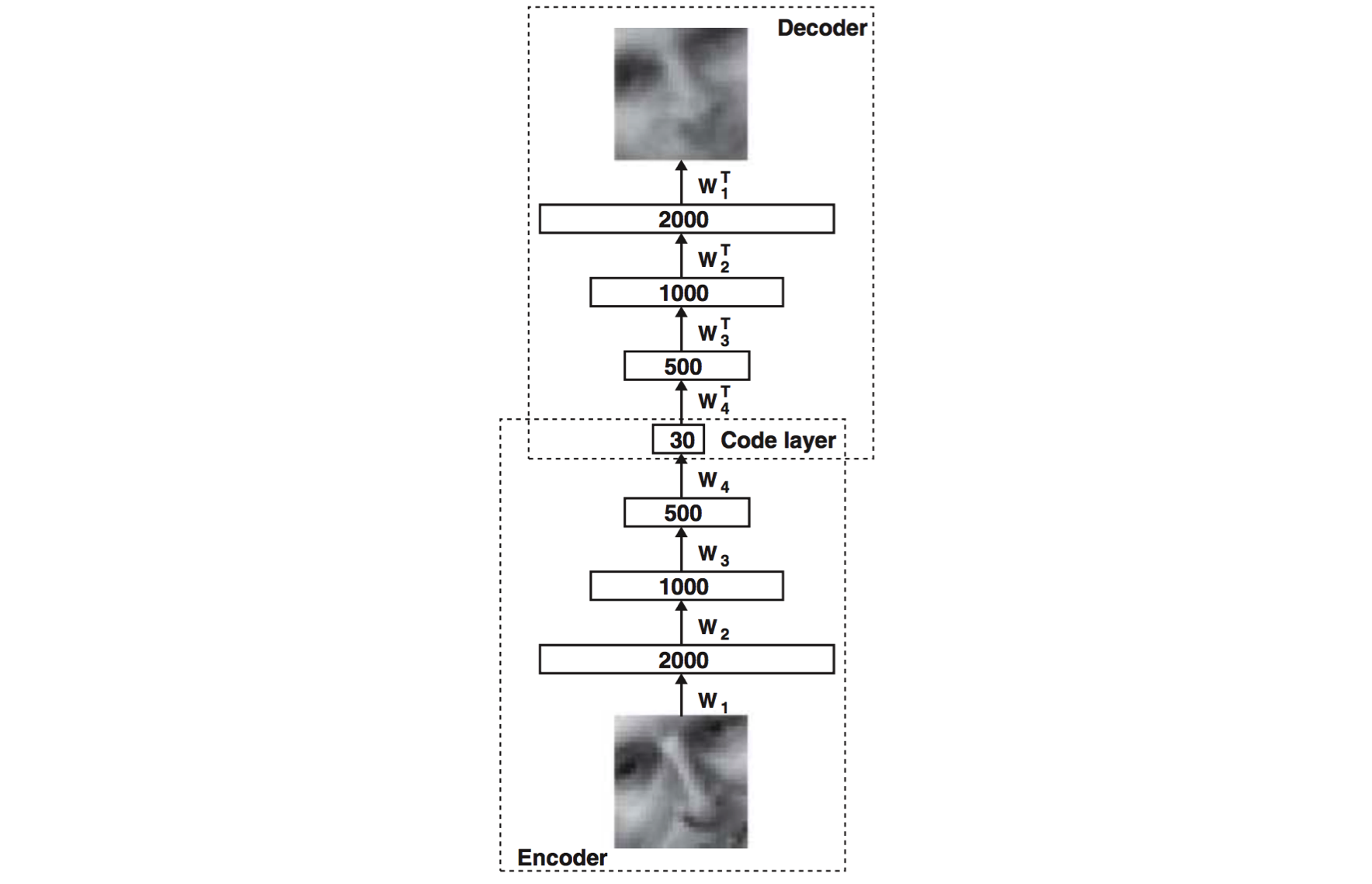
The basic structure of an autoencoder
An autoencoder consists of two major parts, the encoder and the decoder networks. The encoder network is used during both training and deployment, while the decoder network is only used
during training. The purpose of the encoder network is to discover a compressed representation of the given input. In this example, we are generating a 30-dimensional representation from a 2000-dimensional input. The purpose of the decoder network, which is
just a reflection of the encoder network, is to reconstruct the original input as closely as possible. It is used during training in order to force the autoencoder to choose the most informative features in its compressed representation. The closer the reconstructed
input is to the original, the better our original representation!
So how does the autoencoder compare to its linear competitors? Let's take a look at a number of experiments performed by Hinton and Salakhutdinov when the technique debuted in
2006. First, we take a look at how well autoencoders can reconstruct their original output compared to PCA using 30 dimensions.
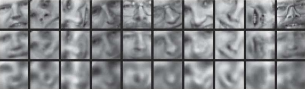
A comparison of reconstruction by an autoencoder (middle) and PCA (bottom) to original image inputs (top)
The reconstruction by the autoencoder is visibly better than the PCA output, which is a very promsing result. We then explore whether autoencoders can significantly improve the separability
of our dataset by comparing 2-dimensional codes produced by an autoencoder to a 2-dimensional representation generated by PCA on the MNIST handwritten digit dataset.
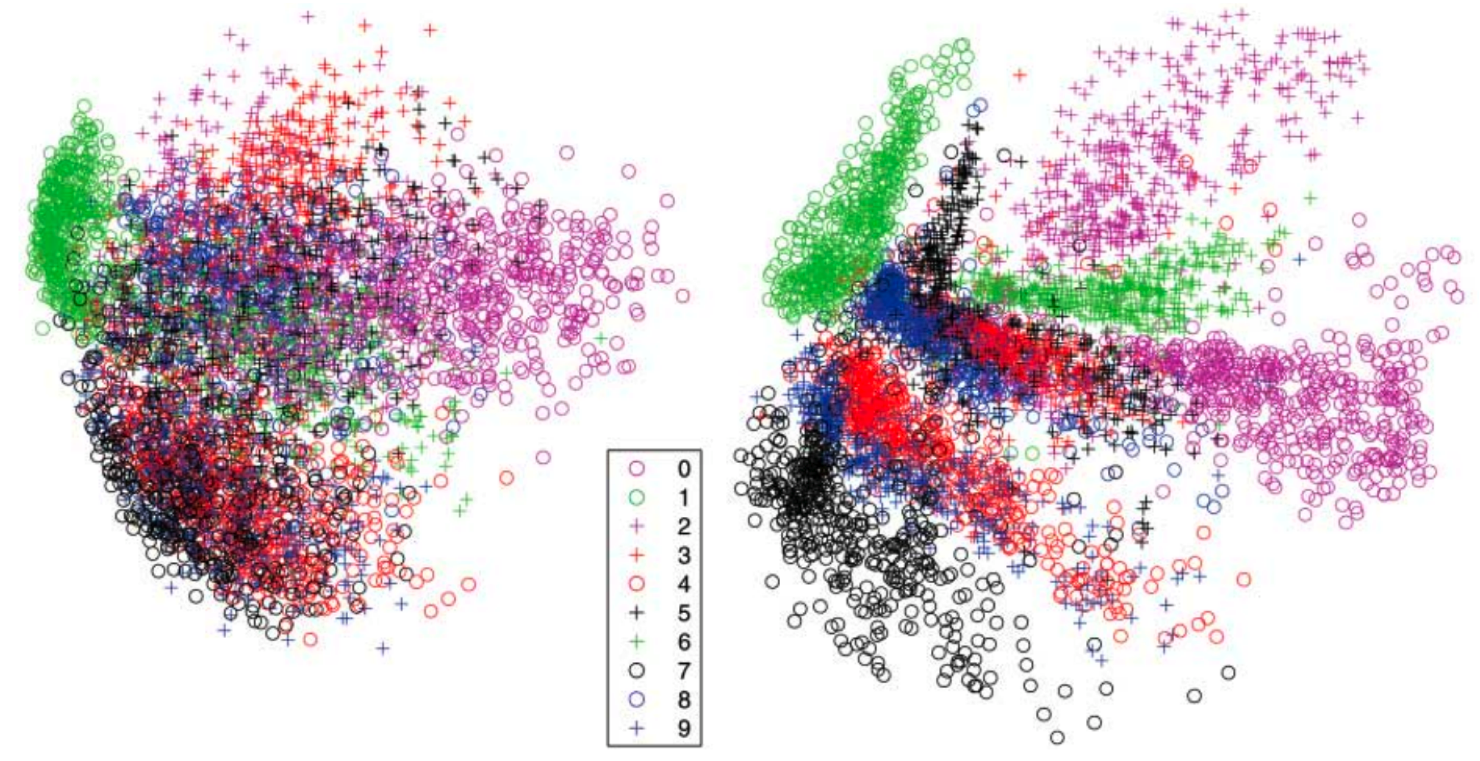
A comparison of separability of 2-dimensional codes generated by an autoencoder (right) and PCA (left) on the MNIST dataset
Finally, we see even more drastic improvements when we compare the autoencoder to the gold-standard unsupervised learning technique for natural language (LSA).
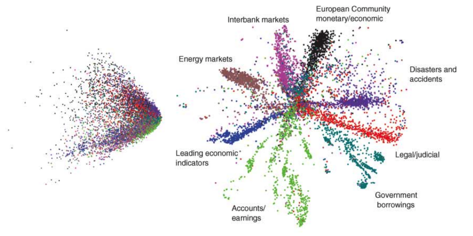
A comparison of separability of 2-dimensional codes generated by an autoencoder (right) and PCA (left) on news stories
made by reseachers handpicking features! We've covered a lot of ground, but we're still only at the tip of the iceberg. In the next blog post, I'll go into much more depth on how autoencoders work, how we efficiently train them, and other clever optimizations
(such as sparsity). If you're interested and would like to talk, please feel free to drop me a line at nkbuduma@gmail.com. I'm always excited to hear new perspectives ❤
from: http://nikhilbuduma.com/2015/03/10/the-curse-of-dimensionality/
as its input and spits out an emotion as an answer. For example, if you passed in the following image, you'd expect the algorithm to label it as "happy."
A greyscale input image of a happy man
Now this is all well and good, but before we're satisfied with this approach, let's take a step back and think about what this really means. A 256 by 256 grayscale image corresponds to
an input vector of over 65,000 dimensions! In other words, we're trying to solve a problem in a 65,000-dimensional space. That's not a particularly easy thing to do, even for a computer! Not only are large inputs annoying to store, move around, and compute
with, but they also give rise to some pretty serious tractability concerns.
Dimensionality is Exponentially Worse
Let's get a rough idea of how the difficulty of a machine learning problem increases as the dimensionality increases. According to astudy byC.J. Stone in 1982, the time it takes to fit a model (specifically a nonparametric regression) to your data is at best proportional to m−p/(2p+d)m−p/(2p+d),
where mm is
the number of data points, dd is
the dimensionality of the data, and pp is
a parameter that depends on the model we are using (specifically, we are assuming that the regression function is pp times
differentiable). In a nutshell, this relation implies that we need exponentially more training examples was we increase the dimensionality of our inputs.
We can observe this graphically by considering a simple example, borrowed from Gutierrez-Osuna. Our learning algorithm divides the feature space uniformly into bins and plot all of our
training examples. We then assign each bin a label based on the predominant class that's found in that bin. Finally, for each new example that we want to classify, we just need to figure out the bin the example falls into and the label associated with that
bin!
In our toy problem, we begin by choosing a single feature (one-dimensional inputs) and divide the space into 3 simple bins:
A simple example involving one-dimensional inputs
Understandably, we notice there's too much overlap between classes, so we decide to add another feature to improve separability. But we notice that if we keep the same number of samples,
we get a 2D scatter plot that's really sparse, and it's really hard to ascertain any meaningful relationships without increasing the number of samples. If we move onto 3-dimensional inputs, it becomes even worse. Now we're trying to fill even more 33=2733=27 bins
with the same number of examples. The scatter plot is nearly empty!
Sparsity becomes exponentially worse as dimension increases
Of important note is that this is NOT an issue that can be easily solved by more effective computing or improved hardware! For many machine learning tasks, collecting training examples
is the most time consuming part, so this mathematical result forces us to be careful about the dimensions we choose to analyze. If we are able to express our inputs in few enough dimensions, we might be able to turn an unfeasible problem into a feasible one!
Manual Feature Selection
Going back to the original problem of classifying facial expressions, it's quite clear that we don't need all 65,000 dimensions to classify an image. Specifically, there are certain key features thatour brain automatically uses to detect emotion quickly. For example, the curve of the person's lips, the extent his brow is furrowed, and the shape of his eyes all help us determine that the man in the picture is feeling happy. It turns out that these features
can be conveniently summarized by looking at the relative positioning of various facial keypoints, and the distances between them.
The key features of human facial expression
Obviously, this allows us to significantly reduce the dimensionality of our input (from 65,000 to about 60), but there are some limitations! Hand selection of features can take years and
years of research to optimize. For many problems, the features that matter are not easy to express. For example, it becomes very difficult to select features for generalized object recognition, where the algorithm needs to tell apart birds, from faces, from
cars, etc. So how do we extract the most information-rich dimensions from our inputs? This is answered by a field of machine learning that is called unsupervised learning. In the next section, we will be discussing the autoencoder, a unsupervised learning
technique pioneered by Geoffrey Hinton that is based on neural networks. We'll briefly talk about how the autoencoder works and how it compares to traditional linear approaches such as principal component analysis (PCA) for computer vision and latent semantic
analysis (LSA) for natural language processing.
A Brief Overview of the Autoencoder
An autoencoder is an unsupervised machine learning technique that utilizes a neural network to produce a low dimensional representation of a high dimensional input. Traditionally, dimensionalityreduction depended on linear methods such as PCA, which finds the directions of maximal variance in high-dimensional data. By selecting only those axes that have the largest variance, PCA aims to capture the directions that contain the most information about
the inputs, so we can express as much as possible with a minimal number of dimensions. The linearity of PCA, however, places significant limitations on the kinds of feature dimensions that can be extracted. Autoencoders overcome these limitations by exploiting
the inherent nonlinearity of neural networks.
The basic structure of an autoencoder
An autoencoder consists of two major parts, the encoder and the decoder networks. The encoder network is used during both training and deployment, while the decoder network is only used
during training. The purpose of the encoder network is to discover a compressed representation of the given input. In this example, we are generating a 30-dimensional representation from a 2000-dimensional input. The purpose of the decoder network, which is
just a reflection of the encoder network, is to reconstruct the original input as closely as possible. It is used during training in order to force the autoencoder to choose the most informative features in its compressed representation. The closer the reconstructed
input is to the original, the better our original representation!
So how does the autoencoder compare to its linear competitors? Let's take a look at a number of experiments performed by Hinton and Salakhutdinov when the technique debuted in
2006. First, we take a look at how well autoencoders can reconstruct their original output compared to PCA using 30 dimensions.
A comparison of reconstruction by an autoencoder (middle) and PCA (bottom) to original image inputs (top)
The reconstruction by the autoencoder is visibly better than the PCA output, which is a very promsing result. We then explore whether autoencoders can significantly improve the separability
of our dataset by comparing 2-dimensional codes produced by an autoencoder to a 2-dimensional representation generated by PCA on the MNIST handwritten digit dataset.
A comparison of separability of 2-dimensional codes generated by an autoencoder (right) and PCA (left) on the MNIST dataset
Finally, we see even more drastic improvements when we compare the autoencoder to the gold-standard unsupervised learning technique for natural language (LSA).
A comparison of separability of 2-dimensional codes generated by an autoencoder (right) and PCA (left) on news stories
Conclusion
Autoencoders are an extremely exciting new approach to unsupervised learning, and for virtually every major kind of machine learning task, they have already surpassed the decades of progressmade by reseachers handpicking features! We've covered a lot of ground, but we're still only at the tip of the iceberg. In the next blog post, I'll go into much more depth on how autoencoders work, how we efficiently train them, and other clever optimizations
(such as sparsity). If you're interested and would like to talk, please feel free to drop me a line at nkbuduma@gmail.com. I'm always excited to hear new perspectives ❤
from: http://nikhilbuduma.com/2015/03/10/the-curse-of-dimensionality/

相关文章推荐
- Android焦点分发基本流程
- C语言标识符
- 萤石Android SDK 集成到AndroidStudio的时候报错,Tag <activity> attribute name has invalid character ' '.
- 左值和右值
- 《圈子圈套2》—— 读后总结
- 面试题3 二维数组中查找
- Java的native方法
- C语言关键字
- 双向链表的应用—实现根据使用频率安排元素位置的功能
- 深度学习整体认识Deep Learning in a Nutshell
- Java 集合转换(数组、List、Set、Map相互转换)
- C++ copy
- LCD电子书项目(四)
- 1002 487-3279(字符串处理)
- NPOI, table string to excel
- jvm 堆、栈、方法区
- java集合:Collection 和 Collections的区别
- Linux系统tcpdump抓包保存cap文件
- 设计模式C++模板方法模式-实际处理交给子类
- 如何获得即时编译器(JIT)的汇编代码(linux环境下)