Class Imbalance Problem
2015-08-24 21:35
309 查看
What is the Class Imbalance Problem?
It is the problem in machine learning where the total number of a class of data (positive) is far less than the total number of another class of data (negative). This problem
is extremely common in practice and can be observed in various disciplines including fraud detection, anomaly detection, medical diagnosis, oil spillage detection, facial recognition, etc.
Why is it a problem?
Most machine learning algorithms and works best when the number of instances of each classes are roughly equal. When the number of instances of one class far exceeds the other, problems arise. This is best illustrated below with an example.
Given a dataset of transaction data, we would like to find out which are fraudulent and which are genuine ones. Now, it is highly cost to the e-commerce company if a fraudulent transaction goes through as this impacts our customers trust in us, and costs us
money. So we want to catch as many fraudulent transactions as possible.
If there is a dataset consisting of 10000 genuine and 10 fraudulent transactions, the classifier will tend to classify fraudulent transactions as genuine transactions. The reason can be easily explained by the numbers. Suppose the machine learning algorithm
has two possibly outputs as follows:
Model 1 classified 7 out of 10 fraudulent transactions as genuine transactions and 10 out of 10000 genuine transactions as fraudulent transactions.
Model 2 classified 2 out of 10 fraudulent transactions as genuine transactions and 100 out of 10000 genuine transactions as fraudulent transactions.
If the classifier’s performance is determined by the number of mistakes, then clearly Model 1 is better as it makes only a total of 17 mistakes while Model 2 made 102 mistakes. However, as we want to minimize the number of fraudulent transactions happening,
we should pick Model 2 instead which only made 2 mistakes classifying the fraudulent transactions. Of course, this could come at the expense of more genuine transactions being classified as fraudulent transactions, but will be a cost we can bear for now. Anyhow,
a general machine learning algorithm will just pick Model 1 than Model 2, which is a problem. In practice, this means we will let a lot of fraudulent transactions go through although we could have stopped them by using Model 2. This translates to unhappy customers
and money lost for the company.
How to tell the machine learning algorithm which is the better solution?
To tell the machine learning algorithm (or the researcher) that Model 2 is better than Model 1, we need to show that Model 2 above is better than Model 1 above. For that, we will need better metrics than just counting the number of mistakes made.
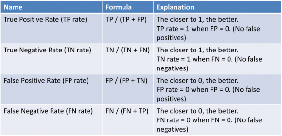
We introduce the concept of True Positive, True Negative, False Positive and False Negative:
True Positive (TP) – An example that is positive and is classified correctly
as positive
True Negative (TN) – An example that is negative and is classified correctly
as negative
False Positive (FP) – An example that is negative but is classified wrongly
as positive
False Negative (FN) – An example that is positive but is classified wrongly
as negative
Based on this above. We will have also the following of True Positive Rate, True Negative Rate, False Positive Rate, False Negative Rate:
With these new metrics, let’s compare it with the conventional metrics of counting the number of mistakes made with the example above. First, we will use the old metrics to calculate the number of mistakes made (error):
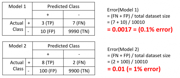
As illustrated above, Model 1 looks like it has lower error (0.1% error) than Model 2 (1.0% error) but we know that Model 2 is the better one, as it makes less false negatives (FN) (maximize true positive (TP)). Now let’s see what the performance of Model 1
and Model 2 are like with the new metrics:
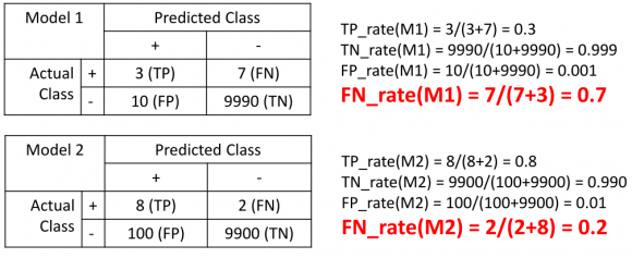
Now, we can see that the false negative rate of Model 1 is at 70% while the false negative rate of Model 2 is just at 20%, which is clearly a better classifier. This is what we should educate the machine learning algorithm (or us) to use in order to allow it
to pick a better algorithm.
How to mitigate this problem?
Now knowing what the Class Imbalance Problem is and why is it a problem, we need to know how to deal with this problem.
We can roughly classify the approaches into two major categories: sampling based approaches and cost function based approaches.
[title3]
Cost function based approaches[/title3]
The intuition behind cost function based approaches is that if we think one false negative is worse than one false positive, we will count that one false negative as, e.g., 100 false negatives instead. For example, if 1 false negative is as costly as 100 false
positives, then the machine learning algorithm will try to make fewer false negatives compared to false positives (since it is cheaper). For example, in the case of SVM, the generic formula is:
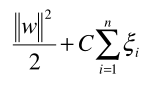
where w is the normal vector to the hyperplane. and E[i] is the error of each data instance, C is
a cost constant and n is the number of data instances. To assign a different cost function to false negative and false positive, we can modify the formula to as follows:
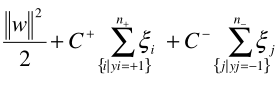
Where C+ is a cost constant for positive cases and C- is a cost constant for negative cases, n+ is
the total number of positive cases and n- is the total number of negative cases. Without diving too deep into the formula above, this is just an example how one may assign different
to cost to positive and negative classes.
[title3]
Sampling based approaches[/title3]
This can be roughly classified into three categories:
Oversampling, by adding more of the minority class so it has more effect on the machine learning algorithm
Undersampling, by removing some of the majority class so it has less effect on the machine learning algorithm
Hybrid, a mix of oversampling and undersampling
However, these approaches have clear drawbacks, as explained below.
[title3]
Undersampling[/title3]
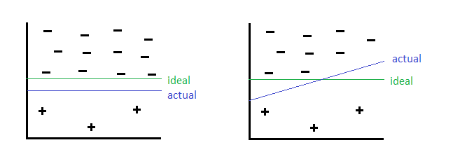
By undersampling, we could risk removing some of the majority class instances which is more representative, thus discarding useful information. This can be illustrated as follows:
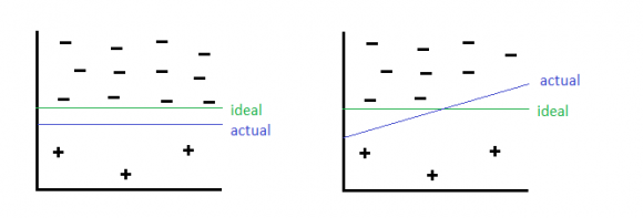
Here the green line is the ideal decision boundary we would like to have, and blue is the actual result. On the left side is the result of just applying a general machine learning algorithm without using undersampling. On the right, we undersampled the negative
class but removed some informative negative class, and caused the blue decision boundary to be slanted, causing some negative class to be classified as positive class wrongly.
[title3]
Oversampling[/title3]
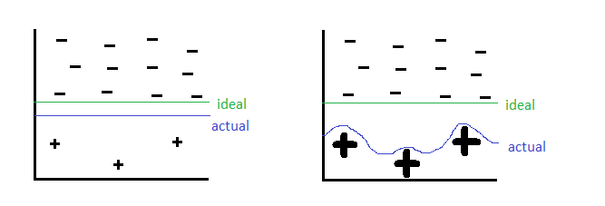
By oversampling, just duplicating the minority classes could lead the classifier to overfitting to a few examples, which can be illustrated below:
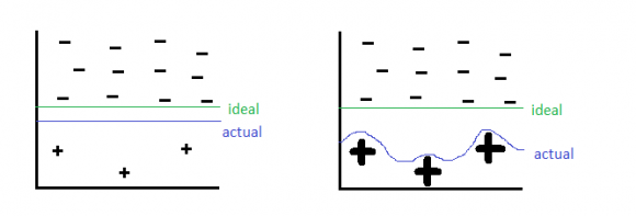
On the left hand side is before oversampling, where as on the right hand side is oversampling has been applied. On the right side, The thick positive signs indicate there are multiple repeated copies of that data instance. The machine learning algorithm then
sees these cases many times and thus designs to overfit to these examples specifically, resulting in a blue line boundary as above.
[title3]
Hybrid approach[/title3]
By combining undersampling and oversampling approaches, we get the advantages but also drawbacks of both approaches as illustrated above, which is still a tradeoff.
[title3]
More recent approaches to the problem[/title3]
In 2002, an sampling based algorithm called SMOTE (Synthetic Minority Over-Sampling Technique) was introduced that try to address the class imbalance problem. It is one of the most adopted approaches due to its simplicity and effectiveness. It is a combination
of oversampling and undersampling, but the oversampling approach is not by replicating minority class but constructing new minority class data instance via an algorithm.
In traditional oversampling, minority class is replicated exactly. In SMOTE, new minority instances are constructed in this way:
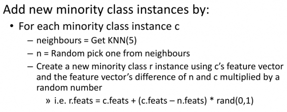
The intuition behind the construction algorithm is that oversampling causes overfit because of repeated instances causes the decision boundary to tighten. Instead, we will create “similar” examples instead. To the machine learning algorithm, these new constructed
instances are not exact copies and thus softens the decision boundary as a result. This be can illustrated as follows:

As a result, the classifier is more general and does not overfit.
[title3]
Even more recent approaches[/title3]
Interested readers may look into more recent literature regarding RUSBoost, SMOTEBagging and Underbagging, which are all regarded as more promising approaches since SMOTE.
However, SMOTE is still very popular due to its simplicity.
Summary
The Class Imbalance Problem is a common problem affecting machine learning due to having disproportionate number of class instances in practice. To compare solutions, we will use alternative metrics (True Positive, True Negative, False Positive, False Negative)
instead of general accuracy of counting number of mistakes.
Due to its prevalence, there are many approaches out there to deal with this problem. They can be generally classified into two major categories of 1) sampling based, and 2) cost function based. Sampling based can be broken into three major categories: a) over
sampling b) under sampling c) hybrid of oversampling and undersampling.
Now armed with what, why and how, you can start dealing with real world scenarios of handling datasets with this problem.
This entry was posted in Machine Learning and
tagged Explain To Me, Machine
Learning on August 30, 2013.


相关文章推荐
- LeetCode263——Ugly Number
- iOS中将汉字转换成拼音的方法
- 解释(n&(n-1))==0的具体含义
- C语言基础--循环 递归打印乘法表
- bootstrap-js(2)下拉菜单
- 可变参数的实现
- PhotoView的异常问题
- 内联函数详解--C++
- 使用Android Studio和Gradle编译NDK项目之Experimental Plugin User Guide
- getopt、getopt_long、getopt_long_only使用实例
- iOS图片轮播
- 大龄屌丝自学笔记--Java零基础到菜鸟--010
- 不等式估计
- 随机生成1-100之间的数,并无一重复的存入长度为100的数组中
- ubuntu 14.04安装opencv3.0.0
- C# windows服务简介
- 八大排序算法
- 找出二进制表示中1的个数相同,且大小最接近的那两个数
- swift详解之十-------------异常处理、类型转换 ( Any and AnyObject )
- poj2112 Optimal Milking --- 最大流量,二分法