NEURAL NETWORKS, PART 2: THE NEURON

NEURAL NETWORKS, PART 2: THE NEURON

A neuron is a very basic classifier. It takes a number of input signals (a feature vector) and outputs a single value (a prediction). A neuron is also a basic building block of neural networks, and by combining together many neurons we can build systems that are capable of learning very complicated patterns. This is part 2 of an introductory series on neural networks. If you haven’t done so yet, you might want to start by learning about the background to neural networks in part 1.

Neurons in artificial neural networks are inspired by biological neurons in nervous systems (shown below). A biological neuron has three main parts: the main body (also known as the soma), dendrites and an axon. There are often many dendrites attached to a neuron body, but only one axon, which can be up to a meter long. In most cases (although there are exceptions), the neuron receives input signals from dendrites, and then outputs its own signals through the axon. Axons in turn connect to the dendrites of other neurons, using special connections called synapses, forming complex neural networks.



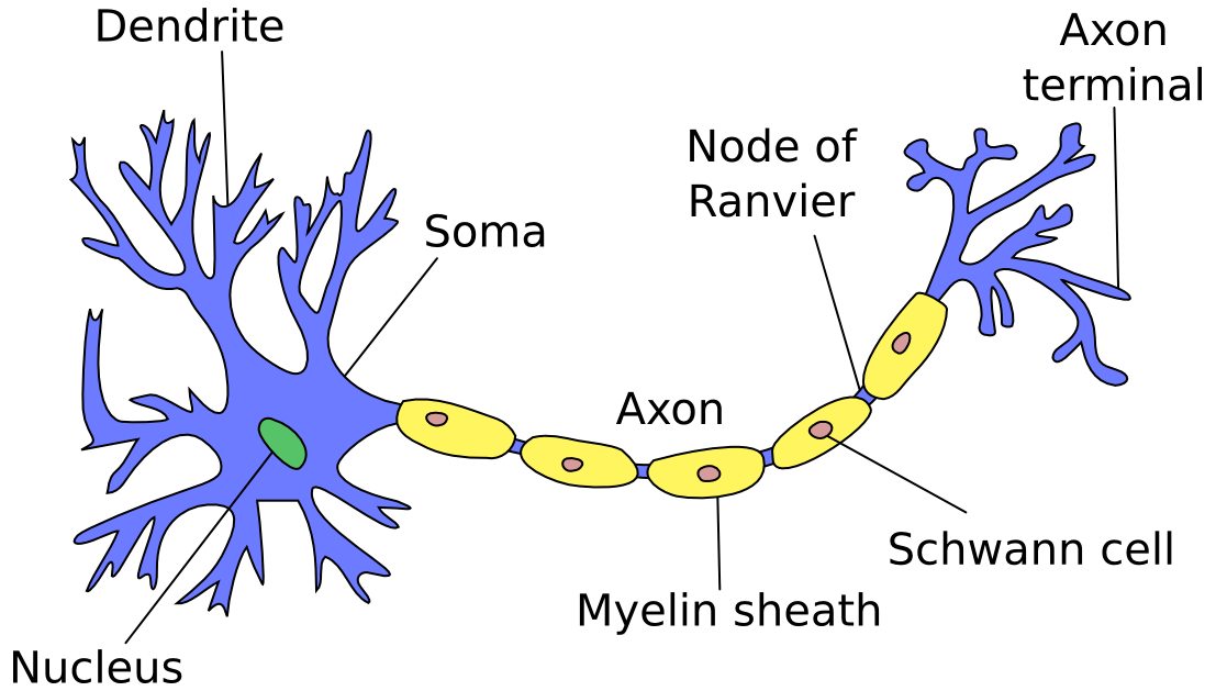
Figure 1: Biological neuron in a nervous system

Below is an illustration of an artificial neuron, where the input is passed in from the left and the prediction comes out from the right. Each input position has a specific weight in the neuron, and they determine what output to give, given a specific input vector. For example, a neuron could be trained to detect cities. We can then take the vector for London from the previous section, give it as input to our neuron, and it will tell us it’s a city by outputting value 1. If we do the same for the word Tuesday, it will give a 0 instead, meaning that it’s not a city.



Figure 2: Artificial neuron

You might notice that there’s a constant value of +1 as one of the input signals, and it has a separate weight w0. This is called a bias, and it allows the network to shift the activation function up or down. Biases are not strictly required for building neurons or neural networks, but they can be very important to the performance, depending on the types of feature values you are using.

Let’s say we have an input vector [1,x1,x2] and a weight vector [w0,w1,w2]. Internally, we first multiply the corresponding input values with their weights, and add them together:

z=(w0×1)+(w1×x1)+(w2×x2)

Then, we pass the sum through an activation function. In this case we will use the sigmoid function (also known as the logistic curve) as our activation function.

y=f(z)=f((w0×1)+(w1×x1)+(w2×x2))

where

f(t)=11+e−t

The sigmoid function takes any real value and maps it to a range between 0 and 1. When plotted, a sigmoid function looks like this:



Figure 3: Sigmoid function

Using a sigmoid as our activation function has some benefits:

Regardless of input, it will map everything to a range between 0 and 1. We don’t have to worry about output values exploding for unexpected input vectors.

The function is non-linear, which allows us to learn more complicated non-linear relationships in our neural networks.

It is differentiable, which comes in handy when we try to perform backpropagation to train our neural networks.

However, it is not required to use an activation function, and there exist many successful network architectures that don’t use one. We could also use a different activation, such as a hyperbolic tangent or a rectifier.

We have now looked at all the components of a neuron, but we’re not going to stop here. Richard Feynman once said “What I cannot create, I do not understand”, so let us create a working example of a neuron. Here is the complete code required to test a neuron with pre-trained weights:

The classify() function is the interesting part in this code. It takes a feature vector as an argument and returns the prediction value y. For testing, we use the examples from the previous section and try to classify each of them. The output of running this code will be as follows:

As you can see, the neuron has successfully separated cities from days. It has also provided a label for the previously-unknown example – apparently the last data point should belong with cities as well.

For this code example, I manually chose and hard-coded weight values, so that it would provide a good classification. In later sections we will see how to have the system learn these values automatically, using some training data.

Now that we know about individual neurons, in the next section we’ll look at how to connect them together and form neural networks.