Sequence of shopping carts in-depth analysis with R(3)– Sequence of events

This is the third part of the sequence of shopping carts in-depth analysis. We processed initial data in the required format, did the exploratory analysis and started the in-depth analysis in

the first post. Finally, we used cluster analysis for creating customer segments in

the second post. As I mentioned in the first post, the sequence can be presented as either state or an event. We dealt with sequences of states until then, which helped us to find some patterns in customers behavior, including time lapses between purchases,
and to create the dummy variable ‘nopurch’ for customers who left us with high probability.

Here, we will focus on analyzing sequences of events that can be helpful as well. We will cover how to find patterns of events. For instance, we will find events that occur systematically together and in the same order, relationships with customers’ characteristics
(typical differences in event sequences between men and women), and association rules between event subsequences.
First of all, we need to create the event sequence object. We can do this easily by converting the state object to event sequince that we already have with the following code:

## [1] (a)-46-(a;b)-24                    
## [2] (a;c)-26-(a;b)-24                  
## [3] (a;c)-20-(a;b;c)-27-(a;b)-20-(a;c)-8
## [4] (a;c)-38-(a)-13-(a;b)-26           
## [5] (a;b)-4-(c)-10-(a;c)-10-(nopurch)-39
## [6] (a;b)-33-(a;b;c)-27-(a;b)-12

As you can see, the df.evseq object includes time lapses and this will allow us to use these data for some custom analysis later.
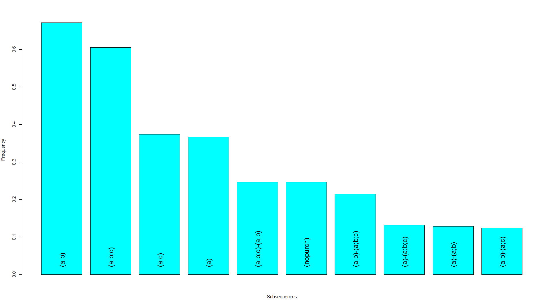
We are starting by searching for frequent event subsequences. A subsequence is formed by a subset of the events and that respects the order of the events in sequence. For instance, (a;b) -> (a) is a subsequence of (a;b) -> (a;b;c)
-> (a) since the order of events are respected. A subsequence is called “frequent” if it occurs in more than a given minimum number of sequences. This required minimum number of sequences to which the subsequence must belong to is called minimum support. It
should be set by us.
Minimum support can be defined in percentages by the pMinSupport argument and in numbers by the minSupport argument. Since our data set is small, we will create a subsequence list object with minimum support 1% and plot the first
10 subsequences with the following code:





In order  to do some custom analysis, in addition to the minimum support, TraMineR also allows to control the search of frequent subsequences with time constraints. For instance, we can specify:
maxGap: maximum time gap between two transitions;
windowSize: maximum window size, that is the maximum time taken by a subsequence;
ageMin: Minimum age at the beginning of the subsequences;
ageMax: Maximum age at the beginning of the subsequences;
ageMaxEnd: Maximum age at the end of the subsequences.
For example, if we want to find the subsequences which are enclosed in a 30 days interval with no more than 10 days between two transitions, we would use the following code:

Furthermore, we can identify the frequent subsequences that are most strongly related with a given factor or find discriminant event subsequences. The discriminant power is evaluated with the p-value of a Chi-square independence
test. The subsequences are then ordered by decreasing the discriminant power. Just as a reminder, in the first post we created the factor variable (df.feat$sex) which consists of the gender of each client. We will search for the subsequences which are related
to gender of client with the following code:

##          Subsequence    Support    p.value statistic index Freq.female
## 1          (a)-(a;c) 0.07612457 0.05445187  3.698792    21  0.05000000
## 2      (a;c)-(a;b;c) 0.12456747 0.06200868  3.482828    11  0.15555556
## 3(a;c)-(a;b;c)-(a;b) 0.02768166 0.06257011  3.467916    37  0.04444444
## 4        (a;c)-(a;c) 0.02768166 0.06626360  3.373233    38  0.01111111
## 5                (a) 0.36678201 0.10055558  2.696710     4  0.32777778
## 6(a)-(a;c)-(nopurch) 0.01038062 0.10127354  2.685372    78  0.00000000
##    Freq.male Resid.female Resid.male
## 1 0.11926606   -1.2703487   1.632473
## 2 0.07339450    1.1779548  -1.513741
## 3 0.00000000    1.3517187  -1.737038
## 4 0.05504587   -1.3362173   1.717118
## 5 0.43119266   -0.8640601   1.110368
## 6 0.02752294   -1.3669353   1.756592
##
## Computed on 289 event sequences
##   Constraint Value
##  countMethod  COBJ

In the resulting plots, the color of each bar is defined by the associated Pearson residual of the Chi-square test. For residuals below -2 (dark red), the subsequence is significantly less frequent than expected under the independence,
whereas for residuals greater than 2 (dark blue), the subsequence is significantly more frequent. We plotted two charts: the first  one displays frequencies, the second one, – residuals. There are several sequences that we can say are related to men and we
need to pay attention to (a) -> (a;c) -> (nopurch) one, because it leads to an increased our customer churn rate.
And finally, we will search for sequential association rules. Association rules learning is a popular and well researched method for discovering relations between variables (subsequences in our case). We will be searching for rules
with the following code:

##              Rules Support      Conf      Lift Standardlift  JMeasure
## 1 (a;b;c) => (a;b)      71 0.4057143 0.6043888    0.2700793 0.2129659
## 2 (a;b) => (a;b;c)      62 0.3195876 0.5277761    0.2069131 0.2404954
## 3   (a) => (a;b;c)      38 0.3584906 0.5920216    0.3571436 0.1789503
## 4     (a) => (a;b)      37 0.3490566 0.5199864    0.3319886 0.3122991
## 5   (a;b) => (a;c)      36 0.1855670 0.4965636    0.3125759 0.1212142
## 6 (a;c) => (a;b;c)      36 0.3333333 0.5504762    0.3319335 0.2176328
##   ImplicStat   p.value p.valueB1 p.valueB2
## 1  1.3809650 0.9163551         1         1
## 2  1.1973199 0.8844091         1         1
## 3  0.6474871 0.7413416         1         1
## 4  2.0592757 0.9802661         1         1
## 5  1.4967428 0.9327699         1         1
## 6  0.9802203 0.8365113         1         1

Here I want you to pay attention. Association rules learning uses a minimum support value as a main parameter (1% in our case). Therefore, you should take this into account when you are calculating the df.subseq variable and defining
the pMinSupport.

As a result, we obtain rules in the if/then format and with several important parameters. For instance, the first one (a;b;c) => (a;b) means: if customer buys the (a;b;c) cart, s/he is likely to also buy the (a;b) cart. The support parameter means that there
are 71 subsequences which contain the (a;b;c) and (a;b) subsequences. The confidence 0.4057 means that in 40.57% of the times a customer buys (a;b;c), (a;b) is bought as well.
Thank you for reading this!