Introduction to LDA (Linear Discrimination Analysis)
2014-10-27 00:22
357 查看
Linear Discrimination Analysis
锻炼一下ability of english writing : ) 光看不写感觉不行哇~
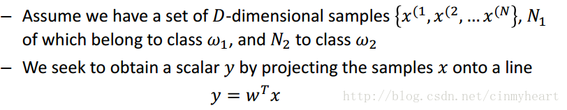
First of all, we try to solve a problem and then guide the LDA out here :)
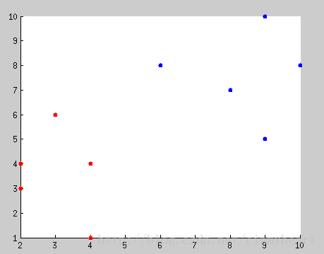
Here is the question that there are two different points in this picture, what's the evidence in mathmatic that you classify there two different points.

After classification, try to input some generic points and classify these inputed points by that mathmatic evidence that you have found.
--------------------------------------------------------------------------------------------------------------------------------------
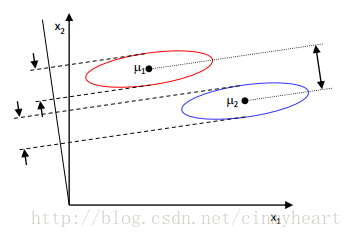
Method One: the distance between projected means
Just compute the different mean value of different class points. Compare the distance between the inputed new points and the mean value's location. If the inputed points is close to mean value location of RED class,
we treat its as red class, verse via.
The green point in this picture is the mean location of blue class.
The yellow point in this picture is the mean location of red class.
Which points close to the mean point of which class, it belongs to that class.

However, the distance between projected means is not a good measure since it does not account for the standard deviation within classes
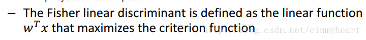
Method two : Fisher’s linear discriminant
This is a fantastic discriminant method \(^o^)/~
What is our target if we want to descriminate different class datas ?
Fisher suggested
maximizing the difference between the means, normalized by a measure of the within-class scatter
Attention! y is a vector but not a normal single dimention varible !

So one of our target is to make the within-class scatter as min as possible.
On the another hand, we should consider about the relationship between the two different class of datas.
If could find a matrix W_t which multiple vector x could translate vectorxinto scaley
, our will finish half of our work.
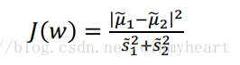
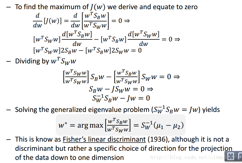
Function J(w) is very helpful. It describe the target of our discriminant. The more bigger of J(w), the better of our discriminant
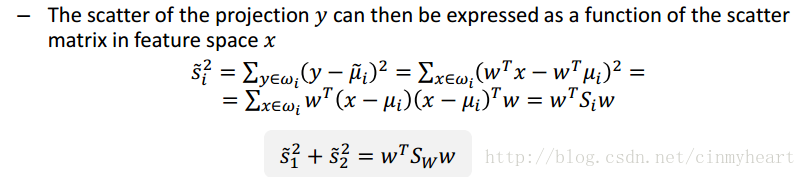
Within-class scatter
Matrix Si describe the level of scatter inner of class-i

Beblow this is a description about within-class scatter in scale y
To get matrix Sw, we could sum all matrix-Si.
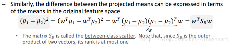
Between-class scatter
This Matrix describe the level of scatter between different class.
Everything is more and more clearly...

At this moment, we may memory back the operation of differential on matrix.
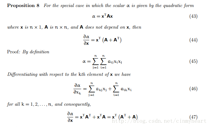
After this, you will have the ability to understand proof beblow here.
Attention! SB is a diagonal
matrix. A_t == A
Let's have a exercise :)
Go back and consider about there data points in below picture.
First of all we should set the data.
And the compute the mean location of each class data collection.
mean_Class_1 =
3.0000 3.6000
mean_Class_2 =
8.4000 7.6000
And then compute S1 and S2
S_w =
13.2000 -2.2000
-2.2000 26.4000
S_b =
29.1600 21.6000
21.6000 16.0000
Look! The red line is what we want! Just project every points onto the red line in the picture.
(y - original_y)/(x - original_x) = -1/slope;
new_location_x = ((1/slope)*x_original_point + y_original_point)/(slope + 1/slope);
new_location_y = slope*new_location_x;
------------------------------------------
update: 2014.10.27
When I look this picture, I doubt that is that projection correctly?
The answer is yes. You could use data in my program . And then you could compute the slope of the blue line and
the slope of original the red point and it's projection point in the blue line.
Multiple that two slope , you must got -1 which means they are verticle with each other.
-------------------------------------------
Now,I will give my code in matlab which draw that picture out here.
锻炼一下ability of english writing : ) 光看不写感觉不行哇~
First of all, we try to solve a problem and then guide the LDA out here :)
Here is the question that there are two different points in this picture, what's the evidence in mathmatic that you classify there two different points.
After classification, try to input some generic points and classify these inputed points by that mathmatic evidence that you have found.
--------------------------------------------------------------------------------------------------------------------------------------
Method One: the distance between projected means
Just compute the different mean value of different class points. Compare the distance between the inputed new points and the mean value's location. If the inputed points is close to mean value location of RED class,
we treat its as red class, verse via.
The green point in this picture is the mean location of blue class.
The yellow point in this picture is the mean location of red class.
Which points close to the mean point of which class, it belongs to that class.
However, the distance between projected means is not a good measure since it does not account for the standard deviation within classes
Method two : Fisher’s linear discriminant
This is a fantastic discriminant method \(^o^)/~
What is our target if we want to descriminate different class datas ?
Fisher suggested
maximizing the difference between the means, normalized by a measure of the within-class scatter
Attention! y is a vector but not a normal single dimention varible !
So one of our target is to make the within-class scatter as min as possible.
On the another hand, we should consider about the relationship between the two different class of datas.
If could find a matrix W_t which multiple vector x could translate vectorxinto scaley
, our will finish half of our work.
Function J(w) is very helpful. It describe the target of our discriminant. The more bigger of J(w), the better of our discriminant
Within-class scatter
Matrix Si describe the level of scatter inner of class-i
Beblow this is a description about within-class scatter in scale y
To get matrix Sw, we could sum all matrix-Si.
Between-class scatter
This Matrix describe the level of scatter between different class.
Everything is more and more clearly...
At this moment, we may memory back the operation of differential on matrix.
After this, you will have the ability to understand proof beblow here.
Attention! SB is a diagonal
matrix. A_t == A
Let's have a exercise :)
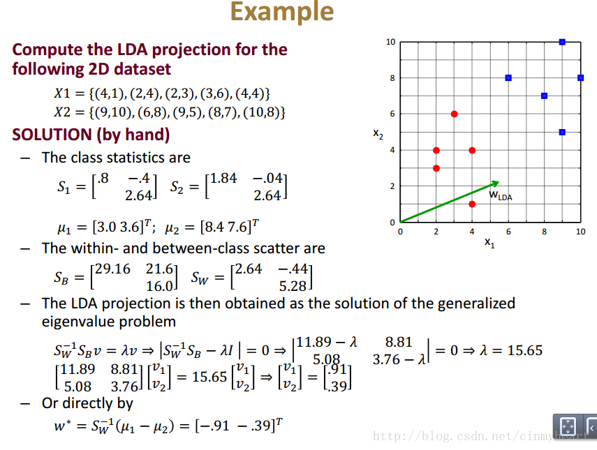
Go back and consider about there data points in below picture.
First of all we should set the data.
Class_1 = [ 4,1;
2,4;
2,3;
3,6;
4,4];

Class_2 = [9,10;
6,8;
9,5;
8,7;
10,8];
And the compute the mean location of each class data collection.
mean_Class_1 = [mean(Class_1(:,1)),mean(Class_1(:,2))];
mean_Class_2 = [mean(Class_2(:,1)),mean(Class_2(:,2))];
mean_Class_1 =
3.0000 3.6000
mean_Class_2 =
8.4000 7.6000
And then compute S1 and S2
S_w =
13.2000 -2.2000
-2.2000 26.4000
S_b =
29.1600 21.6000
21.6000 16.0000
S_w = S_1 + S_2;

S_b = (mean_Class_1 - mean_Class_2)' * (mean_Class_1 - mean_Class_2);
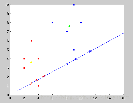
Look! The red line is what we want! Just project every points onto the red line in the picture.
(y - original_y)/(x - original_x) = -1/slope;
new_location_x = ((1/slope)*x_original_point + y_original_point)/(slope + 1/slope);
new_location_y = slope*new_location_x;
------------------------------------------
update: 2014.10.27
When I look this picture, I doubt that is that projection correctly?
The answer is yes. You could use data in my program . And then you could compute the slope of the blue line and
the slope of original the red point and it's projection point in the blue line.
Multiple that two slope , you must got -1 which means they are verticle with each other.
-------------------------------------------
Now,I will give my code in matlab which draw that picture out here.
clear all
close all
clc

Class_1 = [ 4,1;
2,4;
2,3;
3,6;
4,4];

Class_2 = [9,10;
6,8;
9,5;
8,7;
10,8];
figure(1);
hold on;
scatter(Class_1(:,1),Class_1(:,2),'fill','r');
scatter(Class_2(:,1),Class_2(:,2),'fill','b');

mean_Class_1 = [mean(Class_1(:,1)),mean(Class_1(:,2))];
mean_Class_2 = [mean(Class_2(:,1)),mean(Class_2(:,2))];
scatter(mean_Class_1(1,1),mean_Class_1(1,2),'fill','y');
scatter(mean_Class_2(1,1),mean_Class_2(1,2),'fill','g');

value = Class_1;

S_1 = [0 0;0 0];

for temp = 1:size(Class_1,1)
value(temp,1) = Class_1(temp,1) - mean_Class_1(1,1);
value(temp,2) = Class_1(temp,2) - mean_Class_1(1,2);

S_1 = S_1 + value(temp,:)'*value(temp,:);
end

S_2 = [0 0;0 0];

for temp = 1:size(Class_1,1)
value(temp,1) = Class_2(temp,1) - mean_Class_2(1,1);
value(temp,2) = Class_2(temp,2) - mean_Class_2(1,2);

S_2 = S_2 + value(temp,:)'*value(temp,:);
end

S_w = S_1 + S_2;

S_b = (mean_Class_1 - mean_Class_2)' * (mean_Class_1 - mean_Class_2);

Temp_matrix = inv(S_w)*S_b;

%% compute the eig dialog matrix by function eig()
[V,D] = eig(Temp_matrix);

eig_value = max(D(:));

Temp_matrix(1,1) = Temp_matrix(1,1) - eig_value;
Temp_matrix(2,2) = Temp_matrix(2,2) - eig_value;

slope = -Temp_matrix(1,1)./Temp_matrix(1,2);

x = [1:16];
y = slope*x;

plot(x,y);

Projection_Class_1(:,1) = ...
(Class_1(:,1).*(1/slope) + Class_1(:,2))./(slope + (1/slope));

Projection_Class_1(:,2) = Projection_Class_1(:,1).*slope;

scatter(Projection_Class_1(:,1),Projection_Class_1(:,2),'r');

Projection_Class_2(:,1) = ...
(Class_2(:,1).*(1/slope) + Class_2(:,2))./(slope + (1/slope));

Projection_Class_2(:,2) = Projection_Class_2(:,1).*slope;

scatter(Projection_Class_2(:,1),Projection_Class_2(:,2),'b');

相关文章推荐
- 线性判别分析(Linear Discriminant Analysis, LDA)算法分析
- LDA(Linear Discriminant Analysis)算法推导和计算方法
- Fisher线性判别分析(Linear Discriminant Analysis,LDA)
- 线性判别分析(Linear Discriminant Analysis, LDA)算法分析
- 线性判别分析(Linear Discriminant Analysis, LDA)算法分析
- 机器学习降维算法二:LDA(Linear Discriminant Analysis)
- Linear discriminant analysis (LDA)学习笔记
- Applying UML and Patterns: An Introduction to Object-Oriented Analysis and Design and Iterative Deve
- Introduction to Linear Algebra Lecture 1
- An Introduction to Function Point Analysis
- 线性判别分析(Linear Discriminant Analysis,LDA)
- 线性判别分析(Linear Discriminant Analysis, LDA)算法分析
- 机器学习降维算法二:LDA(Linear Discriminant Analysis)
- Introduction to Algorithm - Summary of Chapter 8 - Sorting in Linear Time
- LDA(Linear Discriminant Analysis)
- Video Introduction to Bayesian Data Analysis, Part 1: What is Bayes?
- LDA (Linear Discriminant Analysis) 线性判别分析
- 线性判别分析(Linear Discriminant Analysis, LDA)算法分析
- 线性判别分析(Linear Discriminant Analysis, LDA)算法分析
- 线性判别式分析-LDA-Linear Discriminant Analysis