Mahout----K-means学习

Mahout学习——K-Means Clustering

K-Means这个词第一次使用是在1967，但是它的思想可以追溯到1957年，它是一种非常简单地基于距离的聚类算法，认为每个Cluster由相似的点组成而这种相似性由距离来衡量，不同Cluster间的点应该尽量不相似，每个Cluster都会有一个“重心”；另外它也是一种排他的算法，即任意点必然属于某一Cluster且只属于该Cluster。当然它的缺点也比较明显，例如：对于孤立点敏感、产生最终聚类之间规模的差距不大。

一、基本思想

1、数学描述

给定d维实数向量(

)，后面就将这个实数向量称作点吧，短！K-Means算法会根据事先制定的参数k，将这些点划分出k个Cluster(k
≤ n)，而划分的标准是最小化点与Cluster重心(均值)的距离平方和，假设这些Cluster为：

，则数学描述如下：


，其中

为第i个Cluster的“重心”(Cluster中所有点的平均值)。
聚类的效果类似下图：



具体可见：http://en.wikipedia.org/wiki/K-means_clustering

2、算法步骤

典型的算法如下，它是一种迭代的算法：
(1)、根据事先给定的k值建立初始划分，得到k个Cluster，比如，可以随机选择k个点作为k个Cluster的重心，又或者用Canopy Clustering得到的Cluster作为初始重心(当然这个时候k的值由Canopy Clustering得结果决定)；
(2)、计算每个点到各个Cluster重心的距离，将它加入到最近的那个Cluster；
(3)、重新计算每个Cluster的重心；
(4)、重复过程2~3，直到各个Cluster重心在某个精度范围内不变化或者达到最大迭代次数。
别看算法简单，很多复杂算法的实际效果或许都不如它，而且它的局部性较好，容易并行化，对大规模数据集很有意义；算法时间复杂度是：O(nkt)，其中：n 是聚类点个数，k 是Cluster个数，t 是迭代次数。

三、并行化策略

K-Means较好地局部性使它能很好的被并行化。第一阶段，生成Cluster的过程可以并行化，各个Slaves读取存在本地的数据集，用上述算法生成Cluster集合，最后用若干Cluster集合生成第一次迭代的全局Cluster集合，然后重复这个过程直到满足结束条件，第二阶段，用之前得到的Cluster进行聚类操作。
用map-reduce描述是：datanode在map阶段读出位于本地的数据集，输出每个点及其对应的Cluster；combiner操作对位于本地包含在相同Cluster中的点进行reduce操作并输出，reduce操作得到全局Cluster集合并写入HDFS。

四、Mahout K-Means Clustering说明

mahout实现了标准K-Means Clustering，思想与前面相同，一共使用了2个map操作、1个combine操作和1个reduce操作，每次迭代都用1个map、1个combine和一个reduce操作得到并保存全局Cluster集合，迭代结束后，用一个map进行聚类操作。可以在mahout-core下的src/main/java中的package：org.apache.mahout.clustering.kmeans中找到相关代码：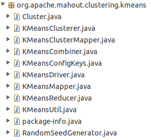

1、数据模型

可以参见上一篇相同标题。

2、目录结构

从目录结构上说，需要两个输入目录：一个用于保存数据点集——input，一个用来保存点的初始划分——clusters；在形成Cluster的阶段，每次迭代会生成一个目录，上一次迭代的输出目录会作为下一次迭代的输入目录，这种目录的命名为：Clusters-“迭代次数”；最终聚类点的结果会放在clusteredPoints文件夹中而Cluster信息放在Clusters-“最后一次迭代次数”文件夹中。

3、如何抽象Cluster

可以从Cluster.java及其父类，对于Cluster，mahout实现了一个抽象类AbstractCluster封装Cluster，具体说明可以参考上一篇文章，这里做个简单说明：
(1）、private int id; #每个K-Means算法产生的Cluster的id
(2）、private long numPoints; #Cluster中包含点的个数，这里的点都是Vector
(3）、private Vector center; #Cluster的重心，这里就是平均值，由s0和s1计算而来。
(4）、private Vector Radius; #Cluster的半径，这个半径是各个点的标准差，反映组内个体间的离散程度，由s0、s1和s2计算而来。
(5）、private double s0; #表示[b]Cluster包含点的权重之和，

[/b]
(6）、private Vector s1; #表示[b]Cluster包含点的加权和，

[/b]
(7）、private Vector s2; #表示[b]Cluster包含点平方的加权和，

[/b]
(8）、public void computeParameters(); #根据s0、s1、s2计算numPoints、center和Radius：













这几个操作很重要，最后三步很必要，在后面会做说明。
(9）、public void observe(VectorWritable x, double weight); #每当有一个新的点加入当前Cluster时都需要更新s0、s1、s2的值
(10)、public ClusterObservation getObservations(); #这个操作在combine操作时会经常被用到，它会返回由s0、s1、s2初始化的ClusterObservation对象，表示当前Cluster中包含的所有被观察过的点

五、K-Means Clustering的Map-Reduce实现

K-Means Clustering的实现同样包含单机版和MR两个版本，单机版就不说了，MR版用了两个map操作、一个combine操作和一个reduce操作，是通过两个不同的job触发，用Dirver来组织的，map和reduce阶段执行顺序是：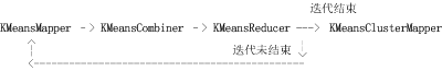

图1

1、初始划分的形成

K-Means算法需要一个对数据点的初始划分，mahout里用了两种方法（以Iris dataset前3个feature为例）：
(1)、使用RandomSeedGenerator类
在指定clusters目录生成k个初始划分并以Sequence File形式存储，其选择方法希望能尽可能不让孤立点作为Cluster重心，大概流程如下：



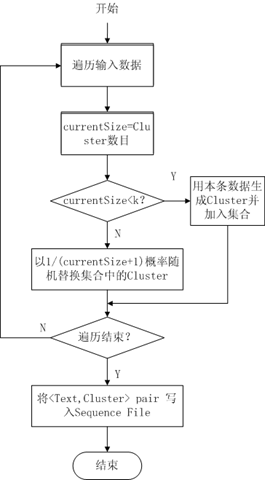
图2
(2)、使用Canopy Clustering
Canopy Clustering常常用来对初始数据做一个粗略的划分，它的结果可以为之后代价较高聚类提供帮助，个人觉得Canopy Clustering用在数据预处理上要比单纯拿来聚类更有用，比如对K-Means来说提供k值，另外还能很好的处理孤立点，当然，需要人工指定的参数由k变成了T1、T2，T1和T2所起的作用是缺一不可的，T1决定了每个Cluster包含点的数目，这直接影响了Cluster的“重心”和“半径”，而T2则决定了Cluster的数目，T2太大会导致只有一个Cluster，而太小则会出现过多的Cluster。通过实验，T1和T2取值会严重影响到算法的效果，如何确定T1和T2，似乎可以用AIC、BIC或者交叉验证去做，但是我没有找到具体做法，希望各位高人给指条明路:)。
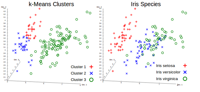
以Iris为例，canopy方法选择T1=3、T2=1.5、cd=0.5、x=10，两种方法结果的前三个维度比较如下：



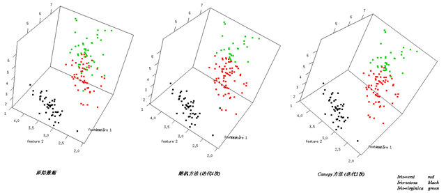
图3
从图中不同Cluster的交界情况可以看出这两种方法的不同效果。

2、配置Cluster信息

K-Means算法的MR实现，第一次迭代需要将随机方法或者Canopy Clustering方法结果目录作为kmeans第一次迭代的输入目录，接下来的每次迭代都需要将上次迭代的输出目录作为本次迭代的输入目录，这就需要能在每次kmeans map和kmeans reduce操作前从该目录得到Cluster的信息，这个功能由KMeansUtil.configureWithClusterInfo实现，它依据指定的HDFS目录将Canopy
Cluster或者上次迭代Cluster的信息存储到一个Collection中，这个方法在之后的每个map和reduce操作中都需要。

3、KMeansMapper

对照上一篇第三节关于MR的那幅图，map操作之前的InputFormat、Split、RR与上一篇完全相同。

1: public class KMeansMapper extends Mapper<WritableComparable<?>, VectorWritable, Text, ClusterObservations> {

2:

3:   private KMeansClusterer clusterer;

4:

5:   private final Collection<Cluster> clusters = new ArrayList<Cluster>();

6:

7:   @Override

8:   protected void map(WritableComparable<?> key, VectorWritable point, Context context)

9:     throws IOException, InterruptedException {

10:     this.clusterer.emitPointToNearestCluster(point.get(), this.clusters, context);

11:   }

12:

13:   @Override

14:   protected void setup(Context context) throws IOException, InterruptedException {

15:     super.setup(context);

16:     Configuration conf = context.getConfiguration();

17:     try {

18:       ClassLoader ccl = Thread.currentThread().getContextClassLoader();

19:       DistanceMeasure measure = ccl.loadClass(conf.get(KMeansConfigKeys.DISTANCE_MEASURE_KEY))

20:           .asSubclass(DistanceMeasure.class).newInstance();

21:       measure.configure(conf);

22:

23:       this.clusterer = new KMeansClusterer(measure);

24:

25:       String clusterPath = conf.get(KMeansConfigKeys.CLUSTER_PATH_KEY);

26:       if (clusterPath != null && clusterPath.length() > 0) {

27:         KMeansUtil.configureWithClusterInfo(conf, new Path(clusterPath), clusters);

28:         if (clusters.isEmpty()) {

29:           throw new IllegalStateException("No clusters found. Check your -c path.");

30:         }

31:       }

32:     } catch (ClassNotFoundException e) {

33:       throw new IllegalStateException(e);

34:     } catch (IllegalAccessException e) {

35:       throw new IllegalStateException(e);

36:     } catch (InstantiationException e) {

37:       throw new IllegalStateException(e);

38:     }

39:   }

40: }

(1)、KMeansMapper接收的是(WritableComparable<?>, VectorWritable) Pair，setup方法利用KMeansUtil.configureWithClusterInfo得到上一次迭代的Clustering结果，map操作需要依据这个结果聚类。
(2)、每个slave机器会分布式的处理存在硬盘上的数据，依据之前得到得Cluster信息，用emitPointToNearestCluster方法将每个点加入到与其距离最近的Cluster，输出结果为(与当前点距离最近Cluster的ID, 由当前点包装而成的ClusterObservations) Pair。

4、KMeansCombiner

combiner操作是一个本地的reduce操作，发生在map之后，reduce之前：

1: public class KMeansCombiner extends Reducer<Text, ClusterObservations, Text, ClusterObservations> {

2:

3:   @Override

4: protected void reduce(Text key, Iterable<ClusterObservations> values, Context context)

5:     throws IOException, InterruptedException {

6:   Cluster cluster = new Cluster();

7:     for (ClusterObservations value : values) {

8:       cluster.observe(value);

9:     }

10:     context.write(key, cluster.getObservations());

11:   }

12:

13: }

5、KMeansReducer

很直白的的操作，只是在setup的时候稍复杂。

1: public class KMeansReducer extends Reducer<Text, ClusterObservations, Text, Cluster> {

2:

3:   private Map<String, Cluster> clusterMap;

4: private double convergenceDelta;

5:   private KMeansClusterer clusterer;

6:

7:   @Override

8:   protected void reduce(Text key, Iterable<ClusterObservations> values, Context context)

9:     throws IOException, InterruptedException {

10:     Cluster cluster = clusterMap.get(key.toString());

11:     for (ClusterObservations delta : values) {

12:     cluster.observe(delta);

13:     }

14:     // force convergence calculation

15:     boolean converged = clusterer.computeConvergence(cluster, convergenceDelta);

16:     if (converged) {

17:       context.getCounter("Clustering", "Converged Clusters").increment(1);

18:     }

19:     cluster.computeParameters();

20:     context.write(new Text(cluster.getIdentifier()), cluster);

21:   }

22:

23:   @Override

24: protected void setup(Context context) throws IOException, InterruptedException {

25:     super.setup(context);

26:     Configuration conf = context.getConfiguration();

27:     try {

28:       ClassLoader ccl = Thread.currentThread().getContextClassLoader();

29:       DistanceMeasure measure = ccl.loadClass(conf.get(KMeansConfigKeys.DISTANCE_MEASURE_KEY))

30:           .asSubclass(DistanceMeasure.class).newInstance();

31:       measure.configure(conf);

32:

33:       this.convergenceDelta = Double.parseDouble(conf.get(KMeansConfigKeys.CLUSTER_CONVERGENCE_KEY));

34:       this.clusterer = new KMeansClusterer(measure);

35:       this.clusterMap = new HashMap<String, Cluster>();

36:

37:       String path = conf.get(KMeansConfigKeys.CLUSTER_PATH_KEY);

38:       if (path.length() > 0) {

39:         Collection<Cluster> clusters = new ArrayList<Cluster>();

40:         KMeansUtil.configureWithClusterInfo(conf, new Path(path), clusters);

41:         setClusterMap(clusters);

42:         if (clusterMap.isEmpty()) {

43:           throw new IllegalStateException("Cluster is empty!");

44:         }

45:       }

46:     } catch (ClassNotFoundException e) {

47:       throw new IllegalStateException(e);

48:     } catch (IllegalAccessException e) {

49:       throw new IllegalStateException(e);

50:     } catch (InstantiationException e) {

51:       throw new IllegalStateException(e);

52:     }

53:   }

54: }

(1)、setup操作的目的是读取初始划分或者上次迭代的结果，构建Cluster信息，同时做了Map<Cluster的ID,Cluster>映射，方便从ID找Cluster。
(2)、reduce操作非常直白，将从combiner传来的<Cluster ID，ClusterObservations>进行汇总；
computeConvergence用来判断当前Cluster是否收敛，即新的“重心”与老的“重心”距离是否满足之前传入的精度要求；
Last but not least，注意到有个cluster.computeParameters()操作，这个操作非常重要，它保证了本次迭代的结果不会影响到下次迭代，也就是保证了能够“重新计算每个Cluster的重心”这一步骤。







前三个操作得到新的Cluster信息；







后三个步骤清空S0、S1、S2信息，保证下次迭代所需的Cluster信息是“干净”的。
之后，reduce将(Cluster ID, Cluster) Pair写入到HDFS中以”clusters-迭代次数“命名的文件夹中。

6、KMeansClusterMapper

之前的MR操作用于构建Cluster信息，KMeansClusterMapper则用构造好的Cluster信息来聚类。

1: public class KMeansClusterMapper

2:   extends Mapper<WritableComparable<?>,VectorWritable,IntWritable,WeightedVectorWritable> {

3:

4: private final Collection<Cluster> clusters = new ArrayList<Cluster>();

5:   private KMeansClusterer clusterer;

6:

7:   @Override

8:   protected void map(WritableComparable<?> key, VectorWritable point, Context context)

9:     throws IOException, InterruptedException {

10:     clusterer.outputPointWithClusterInfo(point.get(), clusters, context);

11:   }

12:

13:   @Override

14:   protected void setup(Context context) throws IOException, InterruptedException {

15:     super.setup(context);

16:     Configuration conf = context.getConfiguration();

17:     try {

18:       ClassLoader ccl = Thread.currentThread().getContextClassLoader();

19:       DistanceMeasure measure = ccl.loadClass(conf.get(KMeansConfigKeys.DISTANCE_MEASURE_KEY))

20:           .asSubclass(DistanceMeasure.class).newInstance();

21:       measure.configure(conf);

22:     

23:       String clusterPath = conf.get(KMeansConfigKeys.CLUSTER_PATH_KEY);

24:     if (clusterPath != null && clusterPath.length() > 0) {

25:         KMeansUtil.configureWithClusterInfo(conf, new Path(clusterPath), clusters);

26:         if (clusters.isEmpty()) {

27:           throw new IllegalStateException("No clusters found. Check your -c path.");

28:         }

29:       }

30:       this.clusterer = new KMeansClusterer(measure);

31:     } catch (ClassNotFoundException e) {

32:     throw new IllegalStateException(e);

33:     } catch (IllegalAccessException e) {

34:       throw new IllegalStateException(e);

35:     } catch (InstantiationException e) {

36:     throw new IllegalStateException(e);

37:     }

38:   }

39: }

(1)、setup依然是从指定目录读取并构建Cluster信息；
(2)、map操作通过计算每个点到各Cluster“重心”的距离完成聚类操作，可以看到map操作结束，所有点就都被放在唯一一个与之距离最近的Cluster中了，因此之后并不需要reduce操作。

7、KMeansDriver

如果把前面的KMeansMapper、KMeansCombiner、KMeansReducer、KMeansClusterMapper看做是砖的话，KMeansDriver就是盖房子的人，它用来组织整个kmeans算法流程(包括单机版和MR版)。示意图如下：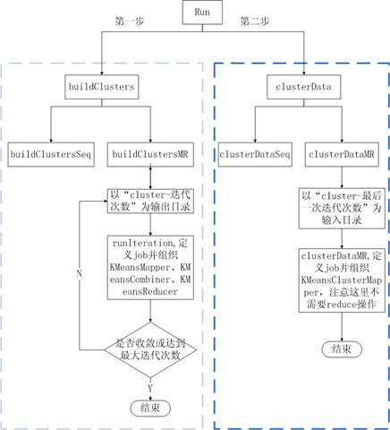


图4

8、Example

在源码的/mahout-examples目录下的package org.apache.mahout.clustering.syntheticcontrol.kmeans中有个Job.java文件提供了对K-Means Clustering的一个版本。核心内容是两个run函数：第一个是用随机选择的方法确定初始划分；第二个是用Canopy 方法确定初始划分，需要注意的是，我们不需要Canopy 方法来做聚类操作，所以CanopyDriver.run的倒数第二个参数(runClustering)要设定为false。
example的使用方法如下：
● 启动master和slave机器；
● 终端输入：hadoop namenode –format
● 终端输入：start-all.sh
● 查看hadoop相关进程是否启动，终端输入：jps
● 在HDFS创建testdata目录，终端输入：hadoop dfs -mkdir testdata
● 将http://archive.ics.uci.edu/ml/中Iris数据集下载，更改一下数据格式，将数据集中“，”替换为“ ”(空格)，并上传到HDFS的testdata文件夹中，进入Iris目录，终端输入：hadoop
dfs -put iris.txt testdata/
● 用Canopy 方法确定初始划分，参数取值为：t1=3，t2=1.5，convergenceDelta=0.5，maxIter=10，进入mahout目录，确认终端执行ls后可以看到mahout-examples-0.5-job.jar这个文件，终端执行：hadoop jar mahout-examples-0.5-job.jar org.apache.mahout.clustering.syntheticcontrol.kmeans.Job
-i testdata -o output -t1 3 -t2 1.5 -cd 0.5 -x 10
● 在http://localhost:50030/jobtracker.jsp 查看作业执行情况：


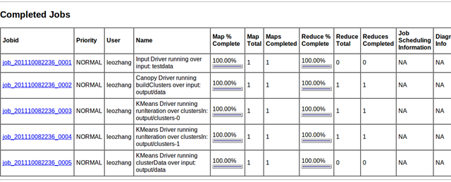
图5

从HDFS上可以看到以下几个目录：



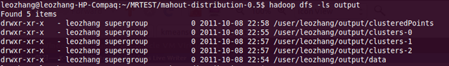
图6
job_201110082236_0001是由InputDriver对原始数据集的一个预处理，输入目录是：testdata，输出目录是：output/data
job_201110082236_0002是由CanopyDriver发起的对data的初始划分，输入目录是：output/data，输出目录是：output/clusters-0
job_201110082236_0003是由KmeansDriver发起的构建Cluster的第一次迭代，输入目录是：output/clusters-0，输出目录是：output/clusters-1
job_201110082236_0004是由KmeansDriver发起的构建Cluster的第二次迭代，输入目录是：output/clusters-1，输出目录是：output/clusters-2
job_201110082236_0005是由KmeansDriver发起的Clustering，输入目录是：output/data，输出目录是：output/clusteredPoints
可见，要查看最终结果需要两个信息：Cluster信息和Clustering data后点的信息，它们分别存储在HDFS的最后一次迭代目录output/clusters-2和聚类点目录output/clusteredPoints。
● 查看结果，将结果获取到本地，终端输入：bin/mahout clusterdump --seqFileDir /user/leozhang/output/clusters-2 --pointsDir /user/leozhang/output/clusteredPoints --output result.txt，终端输入：ls可以看到result.txt这个文件，文件内容类似：

1: VL-1{n=68 c=[5.974, 2.771, 4.501, 1.472] r=[0.471, 0.291, 0.523, 0.303]}

2:   Weight:  Point:

3:  1.0: [7.000, 3.200, 4.700, 1.400]

4:   1.0: [6.400, 3.200, 4.500, 1.500]

5:     1.0: [6.900, 3.100, 4.900, 1.500]

6:   1.0: [5.500, 2.300, 4.000, 1.300]

7:     1.0: [6.500, 2.800, 4.600, 1.500]

8:     1.0: [5.700, 2.800, 4.500, 1.300]

9:     1.0: [6.300, 3.300, 4.700, 1.600]

10:     1.0: [4.900, 2.400, 3.300, 1.000]

11:     1.0: [6.600, 2.900, 4.600, 1.300]

12:   1.0: [5.200, 2.700, 3.900, 1.400]

13:     1.0: [5.000, 2.000, 3.500, 1.000]

14:     1.0: [5.900, 3.000, 4.200, 1.500]

15:     1.0: [6.000, 2.200, 4.000, 1.000]

16:     1.0: [6.100, 2.900, 4.700, 1.400]

17:     1.0: [5.600, 2.900, 3.600, 1.300]

18:     1.0: [6.700, 3.100, 4.400, 1.400]

19:     1.0: [5.600, 3.000, 4.500, 1.500]

20:     1.0: [5.800, 2.700, 4.100, 1.000]

21:     1.0: [6.200, 2.200, 4.500, 1.500]

22:   1.0: [5.600, 2.500, 3.900, 1.100]

23:     1.0: [5.900, 3.200, 4.800, 1.800]

24:   1.0: [6.100, 2.800, 4.000, 1.300]

25:     1.0: [6.300, 2.500, 4.900, 1.500]

26:     1.0: [6.100, 2.800, 4.700, 1.200]

27:     1.0: [6.400, 2.900, 4.300, 1.300]

28:     1.0: [6.600, 3.000, 4.400, 1.400]

29:     1.0: [6.800, 2.800, 4.800, 1.400]

30:     1.0: [6.700, 3.000, 5.000, 1.700]

31:     1.0: [6.000, 2.900, 4.500, 1.500]

32:   1.0: [5.700, 2.600, 3.500, 1.000]

33:     1.0: [5.500, 2.400, 3.800, 1.100]

34:     1.0: [5.500, 2.400, 3.700, 1.000]

35:     1.0: [5.800, 2.700, 3.900, 1.200]

36:   1.0: [6.000, 2.700, 5.100, 1.600]

37:     1.0: [5.400, 3.000, 4.500, 1.500]

38:     1.0: [6.000, 3.400, 4.500, 1.600]

39:     1.0: [6.700, 3.100, 4.700, 1.500]

40:     1.0: [6.300, 2.300, 4.400, 1.300]

41:     1.0: [5.600, 3.000, 4.100, 1.300]

42:     1.0: [5.500, 2.500, 4.000, 1.300]

43:     1.0: [5.500, 2.600, 4.400, 1.200]

44:     1.0: [6.100, 3.000, 4.600, 1.400]

45:     1.0: [5.800, 2.600, 4.000, 1.200]

46:     1.0: [5.000, 2.300, 3.300, 1.000]

47:     1.0: [5.600, 2.700, 4.200, 1.300]

48:     1.0: [5.700, 3.000, 4.200, 1.200]

49:     1.0: [5.700, 2.900, 4.200, 1.300]

50:     1.0: [6.200, 2.900, 4.300, 1.300]

51:     1.0: [5.100, 2.500, 3.000, 1.100]

52:     1.0: [5.700, 2.800, 4.100, 1.300]

53:     1.0: [5.800, 2.700, 5.100, 1.900]

54:     1.0: [4.900, 2.500, 4.500, 1.700]

55:     1.0: [5.700, 2.500, 5.000, 2.000]

56:     1.0: [5.800, 2.800, 5.100, 2.400]

57:     1.0: [6.000, 2.200, 5.000, 1.500]

58:     1.0: [5.600, 2.800, 4.900, 2.000]

59:     1.0: [6.300, 2.700, 4.900, 1.800]

60:     1.0: [6.200, 2.800, 4.800, 1.800]

61:     1.0: [6.100, 3.000, 4.900, 1.800]

62:     1.0: [6.300, 2.800, 5.100, 1.500]

63:     1.0: [6.100, 2.600, 5.600, 1.400]

64:     1.0: [6.000, 3.000, 4.800, 1.800]

65:     1.0: [5.800, 2.700, 5.100, 1.900]

66:     1.0: [6.300, 2.500, 5.000, 1.900]

67:     1.0: [5.900, 3.000, 5.100, 1.800]

68: VL-0{n=51 c=[5.008, 3.400, 1.494, 0.261] r=[0.346, 0.395, 0.273, 0.159]}

69:     Weight:  Point:

70:     1.0: [5.100, 3.500, 1.400, 0.200]

71:     1.0: [4.900, 3.000, 1.400, 0.200]

72:     1.0: [4.700, 3.200, 1.300, 0.200]

73:     1.0: [4.600, 3.100, 1.500, 0.200]

74:     1.0: [5.000, 3.600, 1.400, 0.200]

75:     1.0: [5.400, 3.900, 1.700, 0.400]

76:     1.0: [4.600, 3.400, 1.400, 0.300]

77:     1.0: [5.000, 3.400, 1.500, 0.200]

78:     1.0: [4.400, 2.900, 1.400, 0.200]

79:     1.0: [4.900, 3.100, 1.500, 0.100]

80:     1.0: [5.400, 3.700, 1.500, 0.200]

81:     1.0: [4.800, 3.400, 1.600, 0.200]

82:     1.0: [4.800, 3.000, 1.400, 0.100]

83:     1.0: [4.300, 3.000, 1.100, 0.100]

84:     1.0: [5.800, 4.000, 1.200, 0.200]

85:     1.0: [5.700, 4.400, 1.500, 0.400]

86:     1.0: [5.400, 3.900, 1.300, 0.400]

87:     1.0: [5.100, 3.500, 1.400, 0.300]

88:     1.0: [5.700, 3.800, 1.700, 0.300]

89:     1.0: [5.100, 3.800, 1.500, 0.300]

90:     1.0: [5.400, 3.400, 1.700, 0.200]

91:     1.0: [5.100, 3.700, 1.500, 0.400]

92:     1.0: [4.600, 3.600, 1.000, 0.200]

93:     1.0: [5.100, 3.300, 1.700, 0.500]

94:     1.0: [4.800, 3.400, 1.900, 0.200]

95:     1.0: [5.000, 3.000, 1.600, 0.200]

96:     1.0: [5.000, 3.400, 1.600, 0.400]

97:     1.0: [5.200, 3.500, 1.500, 0.200]

98:     1.0: [5.200, 3.400, 1.400, 0.200]

99:     1.0: [4.700, 3.200, 1.600, 0.200]

100:     1.0: [4.800, 3.100, 1.600, 0.200]

101:     1.0: [5.400, 3.400, 1.500, 0.400]

102:     1.0: [5.200, 4.100, 1.500, 0.100]

103:     1.0: [5.500, 4.200, 1.400, 0.200]

104:     1.0: [4.900, 3.100, 1.500, 0.100]

105:     1.0: [5.000, 3.200, 1.200, 0.200]

106:     1.0: [5.500, 3.500, 1.300, 0.200]

107:     1.0: [4.900, 3.100, 1.500, 0.100]

108:     1.0: [4.400, 3.000, 1.300, 0.200]

109:     1.0: [5.100, 3.400, 1.500, 0.200]

110:     1.0: [5.000, 3.500, 1.300, 0.300]

111:     1.0: [4.500, 2.300, 1.300, 0.300]

112:     1.0: [4.400, 3.200, 1.300, 0.200]

113:     1.0: [5.000, 3.500, 1.600, 0.600]

114:     1.0: [5.100, 3.800, 1.900, 0.400]

115:     1.0: [4.800, 3.000, 1.400, 0.300]

116:     1.0: [5.100, 3.800, 1.600, 0.200]

117:     1.0: [4.600, 3.200, 1.400, 0.200]

118:     1.0: [5.300, 3.700, 1.500, 0.200]

119:     1.0: [5.000, 3.300, 1.400, 0.200]

120: VL-2{n=31 c=[6.932, 3.106, 5.855, 2.142] r=[0.491, 0.293, 0.449, 0.235]}

121:     Weight:  Point:

122:     1.0: [6.300, 3.300, 6.000, 2.500]

123:     1.0: [7.100, 3.000, 5.900, 2.100]

124:     1.0: [6.300, 2.900, 5.600, 1.800]

125:     1.0: [6.500, 3.000, 5.800, 2.200]

126:     1.0: [7.600, 3.000, 6.600, 2.100]

127:     1.0: [7.300, 2.900, 6.300, 1.800]

128:     1.0: [6.700, 2.500, 5.800, 1.800]

129:     1.0: [7.200, 3.600, 6.100, 2.500]

130:     1.0: [6.500, 3.200, 5.100, 2.000]

131:     1.0: [6.400, 2.700, 5.300, 1.900]

132:     1.0: [6.800, 3.000, 5.500, 2.100]

133:     1.0: [6.400, 3.200, 5.300, 2.300]

134:     1.0: [6.500, 3.000, 5.500, 1.800]

135:     1.0: [7.700, 3.800, 6.700, 2.200]

136:     1.0: [7.700, 2.600, 6.900, 2.300]

137:     1.0: [6.900, 3.200, 5.700, 2.300]

138:     1.0: [7.700, 2.800, 6.700, 2.000]

139:     1.0: [6.700, 3.300, 5.700, 2.100]

140:     1.0: [7.200, 3.200, 6.000, 1.800]

141:     1.0: [6.400, 2.800, 5.600, 2.100]

142:     1.0: [7.200, 3.000, 5.800, 1.600]

143:     1.0: [7.400, 2.800, 6.100, 1.900]

144:     1.0: [7.900, 3.800, 6.400, 2.000]

145:     1.0: [6.400, 2.800, 5.600, 2.200]

146:     1.0: [7.700, 3.000, 6.100, 2.300]

147:     1.0: [6.300, 3.400, 5.600, 2.400]

148:     1.0: [6.400, 3.100, 5.500, 1.800]

149:     1.0: [6.900, 3.100, 5.400, 2.100]

150:     1.0: [6.700, 3.100, 5.600, 2.400]

151:     1.0: [6.900, 3.100, 5.100, 2.300]

152:     1.0: [6.800, 3.200, 5.900, 2.300]

153:     1.0: [6.700, 3.300, 5.700, 2.500]

154:     1.0: [6.700, 3.000, 5.200, 2.300]

155:     1.0: [6.500, 3.000, 5.200, 2.000]

156:     1.0: [6.200, 3.400, 5.400, 2.300]

● 为了能比较直观的查看数据，可以利用R(可以使用强大的RStudio，需要安装rgl)，我将数据整理到以下链接：http://files.cnblogs.com/vivounicorn/data%26result.rar ，分组显示数据前三维，不同Cluster用不同颜色表示。效果类似于图3，代码类似于：

1: library(rgl)

2: ttt = textConnection("

3: x      y      z       t       group

4:5.100  3.500  1.400  0.200   Iris-setosa

5:  ．．．．．．．．．

6:6.300  3.300  6.000  2.500   Iris-virginica

7:  ．．．．．．．．．

8:  7.000  3.200  4.700  1.400   Iris-versicolor

9:  ．．．．．．．．．

10: ")

11:

12: colors =c("red","green","blue")

13: pca <- read.table(ttt,header=TRUE)

14: p3d <- plot3d(pca$x, pca$y, pca$z, xlab="feature 1", ylab="feature 2",

15: zlab="feature 3",

16: col=as.integer(pca$group) ,

17: box=FALSE, size=5)

执行pca <- read.table(ttt,header=TRUE)可能会报错：Error in read.table(ttt, header = TRUE) : more columns than column names，没关系，再重新执行一下这句就行了。

六、总结

K-Means Clustering是基于距离的排他的划分方法，初始划分对它很重要，mahout里实现了两种方法：随机方法和Canopy方法，前者比较简单，但孤立点会对其Clustering效果造成较大影响，后者对孤立点的处理能力很强但是需要确定的参数多了一个且如何合理取值需要探讨。

七、参考资料

1、http://mahout.apache.org/

2、https://cwiki.apache.org/MAHOUT/k-means-clustering.html

3、http://developer.yahoo.com/hadoop/tutorial/

4、http://www.ibm.com/developerworks/cn/web/1103_zhaoct_recommstudy3/

5、http://grepcode.com/file/repo1.maven.org/maven2/org.apache.mahout/mahout-utils/0.5/org/apache/mahout/clustering/conversion/InputDriver.java#InputDriver
6、http://faculty.chass.ncsu.edu/garson/PA765/cluster.htm

分类: 机器学习