Linear Decoders
2014-02-21 22:10
351 查看
博文参考standford UFLDL网页教程线性解码器。
1、线性解码器
前面说过的稀疏自编码器是一个三层的feed-forward神经网络结构,包含输入层、隐含层和输出层,隐含层和输出层采用的激活函数都是sigmoid函数,由于sigmoid函数的y值范围在[0,1],这就要求输入也要在这个范围内,MNIST数据是在这个范围内的,但是对于有些数据,我们不知道用什么办法缩放到[0,1]才合适,所以就有线性解码器。线性解码器(linear decoders)其实就是输出层采用线性激活函数,最简单的线性激活函数就是恒等激活函数,就是a=f(z)=z。但是中间隐含层必须采用sigmoid函数或者tanh函数,这两个都是对输入的非线性变换,如果采用线性变换,一方面表达能力没有那么强,另一方面就是没有必要采用三层结构了,直接隐含层当做输出层也可以学到一样的函数关系。有了线性解码器之后,输入层的单元就没必要限制在[0,1]了。
线性解码器的输出层可以通过调整W2使得输出数值可以大于1或者小于0。
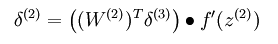
对于线性解码器,当输出层的激活函数变为恒等激活函数,输出单元的误差项变为:
使用BP算法计算隐含层单元的误差为:
2、Learning color features with Sparse Autoencoders
关于实验的一些说明:
实验的数据集是STL-10数据,是RGB三通道图,之前的实验用的是MNIST数据集,MNIST是灰度图;STL-10数据是把RGB组成一个长向量,这样就跟MNIST数据一样了。实验数据patches的大小是192*100000,因为RGB patches大小是8x8,把RGB组合起来就是192.
数据预处理是ZCAWhiten,ZCAWhiten并没有对像PCAWhiten那样对数据进行降维,ZCAWhiten可以得到尽量接近原始数据,但是数据维度之间没有相关性,而且维度的方差一样。
比较奇怪的是最后显示学到的权重图时,代码是displayColorNetwork( (W*ZCAWhite)'),我的理解由于输入一个样本x时,得到的特征是W*ZCAWhite*x,它要显示的是W*ZCAWhite这个变换,如果是把ZCAWhite*x当做原始输入,就跟以前的直接显示W一样了。
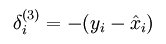
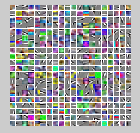
实验结果:
最终学到的特征图为:
Matlab代码把sparseAutoencoderCost.m的代码复制到sparseAutoencoderLinearCost.m并修改几行即可.
1、线性解码器
前面说过的稀疏自编码器是一个三层的feed-forward神经网络结构,包含输入层、隐含层和输出层,隐含层和输出层采用的激活函数都是sigmoid函数,由于sigmoid函数的y值范围在[0,1],这就要求输入也要在这个范围内,MNIST数据是在这个范围内的,但是对于有些数据,我们不知道用什么办法缩放到[0,1]才合适,所以就有线性解码器。线性解码器(linear decoders)其实就是输出层采用线性激活函数,最简单的线性激活函数就是恒等激活函数,就是a=f(z)=z。但是中间隐含层必须采用sigmoid函数或者tanh函数,这两个都是对输入的非线性变换,如果采用线性变换,一方面表达能力没有那么强,另一方面就是没有必要采用三层结构了,直接隐含层当做输出层也可以学到一样的函数关系。有了线性解码器之后,输入层的单元就没必要限制在[0,1]了。
线性解码器的输出层可以通过调整W2使得输出数值可以大于1或者小于0。
对于线性解码器,当输出层的激活函数变为恒等激活函数,输出单元的误差项变为:
使用BP算法计算隐含层单元的误差为:
2、Learning color features with Sparse Autoencoders
关于实验的一些说明:
实验的数据集是STL-10数据,是RGB三通道图,之前的实验用的是MNIST数据集,MNIST是灰度图;STL-10数据是把RGB组成一个长向量,这样就跟MNIST数据一样了。实验数据patches的大小是192*100000,因为RGB patches大小是8x8,把RGB组合起来就是192.
数据预处理是ZCAWhiten,ZCAWhiten并没有对像PCAWhiten那样对数据进行降维,ZCAWhiten可以得到尽量接近原始数据,但是数据维度之间没有相关性,而且维度的方差一样。
比较奇怪的是最后显示学到的权重图时,代码是displayColorNetwork( (W*ZCAWhite)'),我的理解由于输入一个样本x时,得到的特征是W*ZCAWhite*x,它要显示的是W*ZCAWhite这个变换,如果是把ZCAWhite*x当做原始输入,就跟以前的直接显示W一样了。
实验结果:
最终学到的特征图为:
Matlab代码把sparseAutoencoderCost.m的代码复制到sparseAutoencoderLinearCost.m并修改几行即可.
function [cost,grad,features] = sparseAutoencoderLinearCost(theta, visibleSize, hiddenSize, ...
lambda, sparsityParam, beta, data)

% visibleSize: the number of input units (probably 64)
% hiddenSize: the number of hidden units (probably 25)
% lambda: weight decay parameter
% sparsityParam: The desired average activation for the hidden units (denoted in the lecture
%                           notes by the greek alphabet rho, which looks like a lower-case "p").
% beta: weight of sparsity penalty term
% data: Our 192x1000000 matrix containing the training data.  So, data(:,i) is the i-th training example.

% The input theta is a vector (because minFunc expects the parameters to be a vector).
% We first convert theta to the (W1, W2, b1, b2) matrix/vector format, so that this
% follows the notation convention of the lecture notes.

W1 = reshape(theta(1:hiddenSize*visibleSize), hiddenSize, visibleSize);
W2 = reshape(theta(hiddenSize*visibleSize+1:2*hiddenSize*visibleSize), visibleSize, hiddenSize);
b1 = theta(2*hiddenSize*visibleSize+1:2*hiddenSize*visibleSize+hiddenSize);
b2 = theta(2*hiddenSize*visibleSize+hiddenSize+1:end);

% Cost and gradient variables (your code needs to compute these values).
% Here, we initialize them to zeros.
cost = 0;
W1grad = zeros(size(W1));
W2grad = zeros(size(W2));
b1grad = zeros(size(b1));
b2grad = zeros(size(b2));

%% ---------- YOUR CODE HERE --------------------------------------
%  Instructions: Compute the cost/optimization objective J_sparse(W,b) for the Sparse Autoencoder,
%                and the corresponding gradients W1grad, W2grad, b1grad, b2grad.
%
% W1grad, W2grad, b1grad and b2grad should be computed using backpropagation.
% Note that W1grad has the same dimensions as W1, b1grad has the same dimensions
% as b1, etc.  Your code should set W1grad to be the partial derivative of J_sparse(W,b) with
% respect to W1.  I.e., W1grad(i,j) should be the partial derivative of J_sparse(W,b)
% with respect to the input parameter W1(i,j).  Thus, W1grad should be equal to the term
% [(1/m) \Delta W^{(1)} + \lambda W^{(1)}] in the last block of pseudo-code in Section 2.2
% of the lecture notes (and similarly for W2grad, b1grad, b2grad).
%
% Stated differently, if we were using batch gradient descent to optimize the parameters,
% the gradient descent update to W1 would be W1 := W1 - alpha * W1grad, and similarly for W2, b1, b2.
%

%矩阵向量化形式实现,速度比不用向量快得多
Jocst = 0; %平方误差
Jweight = 0; %规则项惩罚
Jsparse = 0; %稀疏性惩罚
[n, m] = size(data); %m为样本数,这里是1000000,n为样本维数,这里是192

%feedforward前向算法计算隐含层和输出层的每个节点的z值(线性组合值)和a值(激活值)
%data每一列是一个样本,
z2 = W1*data + repmat(b1,1,m); %W1*data的每一列是每个样本的经过权重W1到隐含层的线性组合值,repmat把列向量b1扩充成m列b1组成的矩阵
a2 = sigmoid(z2);
z3 = W2*a2 + repmat(b2,1,m);
%%%%对于线性解码器,要修改下面一行%%%%
%a3 = sigmoid(z3);
a3 = z3;
%%%%%%%%%%%%%%%%%%%%

%计算预测结果与理想结果的平均误差
Jcost = (0.5/m)*sum(sum((a3-data).^2));
%计算权重惩罚项
Jweight = (1/2)*(sum(sum(W1.^2))+sum(sum(W2.^2)));
%计算稀疏性惩罚项
rho_hat = (1/m)*sum(a2,2);
Jsparse = sum(sparsityParam.*log(sparsityParam./rho_hat)+(1-sparsityParam).*log((1-sparsityParam)./(1-rho_hat)));

%计算总损失函数
cost = Jcost + lambda*Jweight + beta*Jsparse;

%%%% 修改下面一行对a3的求导%%%%%
%反向传播求误差值
%delta3 = -(data-a3).*fprime(a3); %每一列是一个样本对应的误差
delta3 = -(data-a3);
%%%%%%%%%%%%%%%%%%%%%%
sterm = beta*(-sparsityParam./rho_hat+(1-sparsityParam)./(1-rho_hat));
delta2 = (W2'*delta3 + repmat(sterm,1,m)).*fprime(a2);

%计算梯度
W2grad = delta3*a2';
W1grad = delta2*data';
W2grad = W2grad/m + lambda*W2;
W1grad = W1grad/m + lambda*W1;
b2grad = sum(delta3,2)/m; %因为对b的偏导是个向量,这里要把delta3的每一列加起来
b1grad = sum(delta2,2)/m;

%%----------------------------------
% %对每个样本进行计算, non-vectorial implementation
% [n m] = size(data);
% a2 = zeros(hiddenSize,m);
% a3 = zeros(visibleSize,m);
% Jcost = 0;    %平方误差项
% rho_hat = zeros(hiddenSize,1);   %隐含层每个节点的平均激活度
% Jweight = 0;  %权重衰减项
% Jsparse = 0;   % 稀疏项代价
%
% for i=1:m
%     %feedforward向前转播
%     z2(:,i) = W1*data(:,i)+b1;
%     a2(:,i) = sigmoid(z2(:,i));
%     z3(:,i) = W2*a2(:,i)+b2;
%     %a3(:,i) = sigmoid(z3(:,i));
%     a3(:,i) = z3(:,i);
%     Jcost = Jcost+sum((a3(:,i)-data(:,i)).*(a3(:,i)-data(:,i)));
%     rho_hat = rho_hat+a2(:,i);  %累加样本隐含层的激活度
% end
%
% rho_hat = rho_hat/m; %计算平均激活度
% Jsparse = sum(sparsityParam*log(sparsityParam./rho_hat) + (1-sparsityParam)*log((1-sparsityParam)./(1-rho_hat))); %计算稀疏代价
% Jweight = sum(W1(:).*W1(:))+sum(W2(:).*W2(:));%计算权重衰减项
% cost = Jcost/2/m + Jweight/2*lambda + beta*Jsparse; %计算总代价
%
% for i=1:m
%     %backpropogation向后传播
%     %delta3 = -(data(:,i)-a3(:,i)).*fprime(a3(:,i));
%     delta3 = -(data(:,i)-a3(:,i));
%     delta2 = (W2'*delta3 +beta*(-sparsityParam./rho_hat+(1-sparsityParam)./(1-rho_hat))).*fprime(a2(:,i));
%
%     W2grad = W2grad + delta3*a2(:,i)';
%     W1grad = W1grad + delta2*data(:,i)';
%     b2grad = b2grad + delta3;
%     b1grad = b1grad + delta2;
% end
% %计算梯度
% W1grad = W1grad/m + lambda*W1;
% W2grad = W2grad/m + lambda*W2;
% b1grad = b1grad/m;
% b2grad = b2grad/m;

% -------------------------------------------------------------------
% After computing the cost and gradient, we will convert the gradients back
% to a vector format (suitable for minFunc).  Specifically, we will unroll
% your gradient matrices into a vector.
grad = [W1grad(:) ; W2grad(:) ; b1grad(:) ; b2grad(:)];

end

%%      Implementation of derivation of f(z)
% f(z) = sigmoid(z) = 1./(1+exp(-z))
% a = 1./(1+exp(-z))
% delta(f) = a.*(1-a)
function dz = fprime(a)
dz = a.*(1-a);
end
%%
%-------------------------------------------------------------------
% Here's an implementation of the sigmoid function, which you may find useful
% in your computation of the costs and the gradients.  This inputs a (row or
% column) vector (say (z1, z2, z3)) and returns (f(z1), f(z2), f(z3)).

function sigm = sigmoid(x)

sigm = 1 ./ (1 + exp(-x));
end
相关文章推荐
- struts2标签
- codeforces 394B Very Beautiful Number
- WINCE5.0/6.0开发环境配置与SDK下载
- php ajax学习
- SDP协议分析
- cvDFT
- GDT/IDT
- CAP理论
- 关于六度分割理论的一点认识
- 用Matlab来将分层制造过程中G代码所表示的单层的加工路径显示出来
- 手把手教程: CentOS 6.5 LVS + KeepAlived 搭建 负载均衡 高可用 集群
- 如何在apache官网下载将将jar包
- 解决protobuf数据丢失bug
- 实现zip压缩解压
- Digital Image Processing 学习笔记3
- DOM 遇到的问题 及解决方法
- Android 学习(三)下: UI 控件
- 2月15日工作记录
- 单选框值得选择
- 深入理解SELinux SEAndroid之二