Android Lesson Six: An Introduction to Texture Filtering
2012-06-02 13:17
671 查看
原文地址:http://www.learnopengles.com/android-lesson-six-an-introduction-to-texture-filtering/
bilinear filtering, and
trilinear filtering using mipmaps.
You’ll learn how to make your textures appear more smooth, as well as the drawbacks that come from smoothing. There are also different ways of
rotating an object, one of which is used in this lesson.

Android Lesson Four: Introducing Basic Texturing.
are applied to triangles and drawn on the screen, so these textures can be drawn in various sizes and orientation. The texture filtering options in OpenGL tell it how to filter the texels onto the pixels of the device, depending on the case.
There are three cases:
Each texel maps onto more than one pixel. This is known as magnification.
Each texel maps exactly onto one pixel. Filtering doesn’t apply in this case.
Each texel maps onto less than one pixel. This is known as minification.
OpenGL lets us assign a filter for both magnification and minification, and lets us use nearest-neighbour, bilinear filtering, or trilinear filtering. I will explain what these mean further below.
Magnification and minification
Here is a visualization of both magnification and minification with nearest-neighbour rendering, using the cute Android that shows up when you have your USB connected to your Android device:

Magnification

As you can see, the texels of the image are easily visible, as they now cover many of the pixels on your display.
Minification

With minification, many of the details are lost as many of the texels cannot be rendered onto the limited pixels available.
Texture filtering modes
Bilinear interpolation
The texels of a texture are clearly visible as large squares in the magnification example when no interpolation between the texel values are done. When rendering is done in
nearest-neighbour mode, the pixel is assigned the value of the nearest texel.
The rendering quality can be dramatically improved by switching to bilinear interpolation. Instead of assigning the values of a group of pixels to the same nearby texel value, these values will instead be linearly interpolated between the neighbouring
four texels. Each pixel will be smoothed out and the resulting image will look much smoother:

Some blockiness is still apparent, but the image looks much smoother than before. People who played 3D games back in the days before 3D accelerated cards came out will remember that this was the defining feature between a software-rendered game and a hardware-accelerated
game: software-rendered games simply did not have the processing budget to do smoothing, so everything appeared blocky and jagged. Things suddenly got smooth once people starting using graphics accelerators.
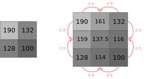
Image via Wikipedia
Bilinear interpolation is mostly useful for magnification. It can also be used for minification, but beyond a certain point and we run into the same problem that we are trying to cram far too many texels onto the same pixel. OpenGL will only use at most
4 texels to render a pixel, so a lot of information is still being lost.
If we look at a detailed texture with bilinear interpolation being applied, it will look very noisy when we see it moving in the distance, since a different set of texels will be selected each frame.
Mipmapping
How can we minify textures without introducing noise and use all of the texels? This can be done by generating a set of optimized textures at different sizes which we can then use at runtime. Since these textures are pre-generated, they can be filtered using
more expensive techniques that use all of the texels, and at runtime OpenGL will select the most appropriate level based on the final size of the texture on the screen.

The resulting image can have more detail, less noise, and look better overall. Although a bit more memory will be used, rendering can also be faster, as the smaller levels can be more easily kept in the GPU’s texture cache. Let’s take a closer look at the
resulting image at 1/8th of its original size, using bilinear filtering without and with mipmaps; the image has been expanded for clarity:
Bilinear filtering without mipmaps

[b]Bilinear filtering with mipmaps[/b]

The version using mipmaps has vastly more detail. Because of the pre-processing of the image into separate levels, all of the texels end up getting used in the final image.
Trilinear filtering
When using mipmaps with bilinear filtering, sometimes a noticeable jump or line can be seen in the rendered scene where OpenGL switches between different mipmap levels of the texture. This will be pointed out a bit further below when comparing the different
OpenGL texture filtering modes.
Trilinear filtering solves this problem by also interpolating between the different mipmap levels, so that a total of 8 texels will be used to interpolate the final pixel value, resulting in a smoother image.
GL_TEXTURE_MIN_FILTER
GL_TEXTURE_MAG_FILTER
These correspond to the minification and magnification described earlier. GL_TEXTURE_MIN_FILTER accepts the following options:
GL_NEAREST
GL_LINEAR
GL_NEAREST_MIPMAP_NEAREST
GL_NEAREST_MIPMAP_LINEAR
GL_LINEAR_MIPMAP_NEAREST
GL_LINEAR_MIPMAP_LINEAR
GL_TEXTURE_MAG_FILTER accepts the following options:
GL_NEAREST
GL_LINEAR
GL_NEAREST corresponds to nearest-neighbour rendering, GL_LINEAR corresponds to bilinear filtering, GL_LINEAR_MIPMAP_NEAREST corresponds to bilinear filtering with mipmaps, and GL_LINEAR_MIPMAP_LINEAR corresponds to trilinear filtering. Graphical examples
and further explanation of the most common options are visible further down in this lesson.
How to set a texture filtering mode
We first need to bind the texture, then we can set the appropriate filter parameter on that texture:
How to generate mipmaps
This is really easy. After loading the texture into OpenGL (See Android Lesson Four: Introducing Basic Texturing for more information
on how to do this), while the texture is still bound, we can simply call:
This will generate all of the mipmap levels for us, and these levels will get automatically used depending on the texture filter set.
downloading the app and giving it a shot.
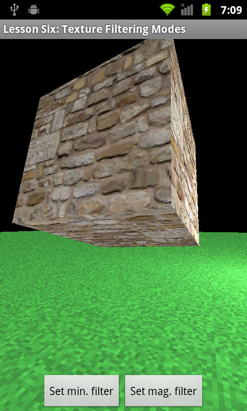
Nearest-neighbour rendering
This mode is reminiscent of older software-rendered 3D games.
GL_TEXTURE_MIN_FILTER = GL_NEAREST
GL_TEXTURE_MAG_FILTER = GL_NEAREST
Bilinear filtering, with mipmaps
This mode was used by many of the first games that supported 3D acceleration and is an efficient way of smoothing textures on Android phones today.
GL_TEXTURE_MIN_FILTER = GL_LINEAR_MIPMAP_NEAREST
GL_TEXTURE_MAG_FILTER = GL_LINEAR

It’s hard to see on this static image, but when things are in motion, you might notice horizontal bands where the rendered pixels switch between mipmap levels.
Trilinear filtering
This mode improves on the render quality of bilinear filtering with mipmaps, by interpolating
between the mipmap levels.
GL_TEXTURE_MIN_FILTER = GL_LINEAR_MIPMAP_LINEAR
GL_TEXTURE_MAG_FILTER = GL_LINEAR

The pixels are completely smoothed between near and far distances; in fact, the textures may now appear too smooth at oblique angles.
Anisotropic filtering is a more advanced technique that is supported by some mobile GPUs and can be used to improve the final results beyond what trilinear filtering
can deliver.
Further exercises
What sort of effects can you achieve with the other modes? For example, when would you use something like GL_NEAREST_MIPMAP_LINEAR?
Android Lesson Six: An Introduction to Texture Filtering
In this lesson, we will introduce the different types of basic texture filtering modes and how to use them, including nearest-neighbour filtering,bilinear filtering, and
trilinear filtering using mipmaps.
You’ll learn how to make your textures appear more smooth, as well as the drawbacks that come from smoothing. There are also different ways of
rotating an object, one of which is used in this lesson.
Assumptions and prerequisites
It’s highly recommended to understand the basics of texture mapping in OpenGL ES, covered in the lessonAndroid Lesson Four: Introducing Basic Texturing.
What is texture filtering?
Textures in OpenGL are made up of arrays of elements known as texels, which contain colour and alpha values. This corresponds with the display, which is made up of a bunch of pixels and displays a different colour at each point. In OpenGL, texturesare applied to triangles and drawn on the screen, so these textures can be drawn in various sizes and orientation. The texture filtering options in OpenGL tell it how to filter the texels onto the pixels of the device, depending on the case.
There are three cases:
Each texel maps onto more than one pixel. This is known as magnification.
Each texel maps exactly onto one pixel. Filtering doesn’t apply in this case.
Each texel maps onto less than one pixel. This is known as minification.
OpenGL lets us assign a filter for both magnification and minification, and lets us use nearest-neighbour, bilinear filtering, or trilinear filtering. I will explain what these mean further below.
Magnification and minification
Here is a visualization of both magnification and minification with nearest-neighbour rendering, using the cute Android that shows up when you have your USB connected to your Android device:
Magnification
As you can see, the texels of the image are easily visible, as they now cover many of the pixels on your display.
Minification
With minification, many of the details are lost as many of the texels cannot be rendered onto the limited pixels available.
Texture filtering modes
Bilinear interpolation
The texels of a texture are clearly visible as large squares in the magnification example when no interpolation between the texel values are done. When rendering is done in
nearest-neighbour mode, the pixel is assigned the value of the nearest texel.
The rendering quality can be dramatically improved by switching to bilinear interpolation. Instead of assigning the values of a group of pixels to the same nearby texel value, these values will instead be linearly interpolated between the neighbouring
four texels. Each pixel will be smoothed out and the resulting image will look much smoother:
Some blockiness is still apparent, but the image looks much smoother than before. People who played 3D games back in the days before 3D accelerated cards came out will remember that this was the defining feature between a software-rendered game and a hardware-accelerated
game: software-rendered games simply did not have the processing budget to do smoothing, so everything appeared blocky and jagged. Things suddenly got smooth once people starting using graphics accelerators.

Image via Wikipedia
Bilinear interpolation is mostly useful for magnification. It can also be used for minification, but beyond a certain point and we run into the same problem that we are trying to cram far too many texels onto the same pixel. OpenGL will only use at most
4 texels to render a pixel, so a lot of information is still being lost.
If we look at a detailed texture with bilinear interpolation being applied, it will look very noisy when we see it moving in the distance, since a different set of texels will be selected each frame.
Mipmapping
How can we minify textures without introducing noise and use all of the texels? This can be done by generating a set of optimized textures at different sizes which we can then use at runtime. Since these textures are pre-generated, they can be filtered using
more expensive techniques that use all of the texels, and at runtime OpenGL will select the most appropriate level based on the final size of the texture on the screen.
The resulting image can have more detail, less noise, and look better overall. Although a bit more memory will be used, rendering can also be faster, as the smaller levels can be more easily kept in the GPU’s texture cache. Let’s take a closer look at the
resulting image at 1/8th of its original size, using bilinear filtering without and with mipmaps; the image has been expanded for clarity:
Bilinear filtering without mipmaps
[b]Bilinear filtering with mipmaps[/b]
The version using mipmaps has vastly more detail. Because of the pre-processing of the image into separate levels, all of the texels end up getting used in the final image.
Trilinear filtering
When using mipmaps with bilinear filtering, sometimes a noticeable jump or line can be seen in the rendered scene where OpenGL switches between different mipmap levels of the texture. This will be pointed out a bit further below when comparing the different
OpenGL texture filtering modes.
Trilinear filtering solves this problem by also interpolating between the different mipmap levels, so that a total of 8 texels will be used to interpolate the final pixel value, resulting in a smoother image.
OpenGL texture filtering modes
OpenGL has two parameters that can be set:GL_TEXTURE_MIN_FILTER
GL_TEXTURE_MAG_FILTER
These correspond to the minification and magnification described earlier. GL_TEXTURE_MIN_FILTER accepts the following options:
GL_NEAREST
GL_LINEAR
GL_NEAREST_MIPMAP_NEAREST
GL_NEAREST_MIPMAP_LINEAR
GL_LINEAR_MIPMAP_NEAREST
GL_LINEAR_MIPMAP_LINEAR
GL_TEXTURE_MAG_FILTER accepts the following options:
GL_NEAREST
GL_LINEAR
GL_NEAREST corresponds to nearest-neighbour rendering, GL_LINEAR corresponds to bilinear filtering, GL_LINEAR_MIPMAP_NEAREST corresponds to bilinear filtering with mipmaps, and GL_LINEAR_MIPMAP_LINEAR corresponds to trilinear filtering. Graphical examples
and further explanation of the most common options are visible further down in this lesson.
How to set a texture filtering mode
We first need to bind the texture, then we can set the appropriate filter parameter on that texture:
GLES20.glBindTexture(GLES20.GL_TEXTURE_2D, mTextureHandle);
GLES20.glTexParameteri(GLES20.GL_TEXTURE_2D, GLES20.GL_TEXTURE_MIN_FILTER, filter);
How to generate mipmaps
This is really easy. After loading the texture into OpenGL (See Android Lesson Four: Introducing Basic Texturing for more information
on how to do this), while the texture is still bound, we can simply call:
GLES20.glGenerateMipmap(GLES20.GL_TEXTURE_2D);
This will generate all of the mipmap levels for us, and these levels will get automatically used depending on the texture filter set.
How does it look?
Here are some screenshots of the most common combinations available. The effects are more dramatic when you see it in motion, so I recommenddownloading the app and giving it a shot.
Nearest-neighbour rendering
This mode is reminiscent of older software-rendered 3D games.
GL_TEXTURE_MIN_FILTER = GL_NEAREST
GL_TEXTURE_MAG_FILTER = GL_NEAREST
Bilinear filtering, with mipmaps
This mode was used by many of the first games that supported 3D acceleration and is an efficient way of smoothing textures on Android phones today.
GL_TEXTURE_MIN_FILTER = GL_LINEAR_MIPMAP_NEAREST
GL_TEXTURE_MAG_FILTER = GL_LINEAR
It’s hard to see on this static image, but when things are in motion, you might notice horizontal bands where the rendered pixels switch between mipmap levels.
Trilinear filtering
This mode improves on the render quality of bilinear filtering with mipmaps, by interpolating
between the mipmap levels.
GL_TEXTURE_MIN_FILTER = GL_LINEAR_MIPMAP_LINEAR
GL_TEXTURE_MAG_FILTER = GL_LINEAR
The pixels are completely smoothed between near and far distances; in fact, the textures may now appear too smooth at oblique angles.
Anisotropic filtering is a more advanced technique that is supported by some mobile GPUs and can be used to improve the final results beyond what trilinear filtering
can deliver.
Further exercises
What sort of effects can you achieve with the other modes? For example, when would you use something like GL_NEAREST_MIPMAP_LINEAR?

相关文章推荐
- Android Lesson Five: An Introduction to Blending
- Android Lesson Eight: An Introduction to Index Buffer Objects (IBOs)
- Android: An introduction to the Edify (Updater-Script) language
- Android Lesson Seven: An Introduction to Vertex Buffer Objects (VBOs)
- An Introduction to Using Binder Framework on Android Operating System
- An Introduction to Delta Sigma Converters (Delta-Sigma转换器 上篇)
- An Introduction to Interactive Programming in Python - Week zero
- Coursera-An Introduction to Interactive Programming in Python (Part 1)-Mini-project— Rock-paper-scissors-lizard-Spock
- An Introduction to Data Mining
- android.view.WindowManager$BadTokenException: Unable to add window--token null is not for an applica
- An introduction to the credit scheduler in Xen
- An Introduction to AJAX Techniques and Frameworks for ASP.NET
- Adding a library/JAR to an Eclipse Android project
- An introduction to C++ Traits
- How to quickly access the source of an “android library project”
- Game Sound: An Introduction to the History, Theory, and Practice of Video Game Music and Sound Desig
- An Introduction to Bioinformatics Algorithms - II - page79 -114
- android.view.WindowManager$BadTokenException: Unable to add window — token null is not for an applic
- Introduction to Windows Filtering Platform Callout Drivers
- Introduction to Android Theme Customization