您的位置：首页 > 编程语言 > Go语言

Laplace方程求解

2012-04-11 09:24 295 查看

Laplace Equation

From Wikiversity

Jump to:
navigation,
search

[hide]
1
Laplace Equation
1.1
Solution to Case with 1 Non-homogeneous Boundary Condition
1.1.1
Step 1: Separate Variables
1.1.2
Step 2: Translate Boundary Conditions
1.1.3
Step 3: Solve the Sturm-Liouville Problem
1.1.4
Step 4: Solve Remaining ODE
1.1.5
Step 5: Combine Solutions

1.2
Solution to Case with 4 Non-homogeneous Boundary Conditions

Laplace Equation[edit]

The Laplace equation is a basic PDE that arises in the heat and diffusion equations. The Laplace equation is defined as:

Solution to Case with 1 Non-homogeneous Boundary Condition[edit]

In a condensed notation in (x,y,z) rectangular coordinates, the Laplace equation in two dimensions reduces to: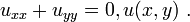

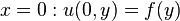
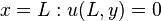
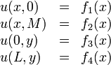
The solution to the case with 1 non-homogeneous boundary condition is the most basic solution type. For the purposes of this example, we consider that the following boundary conditions hold true for this equation:

Step 1: Separate Variables[edit]

To solve this equation, we assume that the function

is comprised of two functions

and

such that

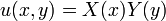
. Hence,

and

Making the substitutions into the Laplace equation, we get:

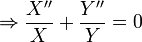
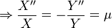
The

is called a separation constant because the solution to the equation must yield a constant. Because of the separation constant,
it yields two linear ODEs:

Step 2: Translate Boundary Conditions[edit]

Translating the boundary conditions allows us to divide the boundary conditions among the variables. This division yields:

Step 3: Solve the Sturm-Liouville Problem[edit]

The last two boundary conditions are homogeneous boundary conditions for the function

. Using the solution to the

Sturm-Liouville problems (SLP), we can easily get a function for

. The following is a fairly simple SLP:

The solution to the SLP yields the following information:

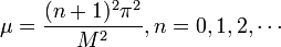
The solution we obtained is a family of solutions dependent on the value for n.

Step 4: Solve Remaining ODE[edit]

The remaining ODE that we have doesn't have a SLP solution to it because we only know one boundary condition for it. We have to use what we obtained from the SLP solution to help us solve this ODE. We obtained the following information from steps 1 and 2:

From analyzing the
second order ODE, we obtain the characteristic equation

Out of the solution set that results from the exponentials, the only viable solution that arises is:

The substitution of (x-L) instead of x in the equation results only in a shift in the eigenspace, so it is valid and it helps us apply the boundary condition. Since

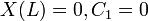
. For convenience, we choose

The resulting equation is:

Step 5: Combine Solutions[edit]

We obtained equations for our separate variable functions and now we can substitute into our assumption in step 1. The substitution yields:

This function only satisfies the 3 homogeneous boundary conditions, however. To solve for the solution to the non-homogeneous boundary condition, we must consider that the complete solution consists of the following infinite series of terms:

At the non-homogeneous boundary condition:

This is an orthogonal expansion of

relative to the orthogonal basis of the sine function. The term

is a Fourier coefficient which is defined as the inner product:

Thus, the coefficient of the infinite series solution

is:

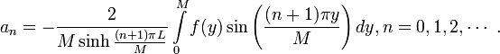
So, the entire general solution to the Laplace equation is:

This is the general solution for the specific set of boundary conditions we assumed at the beginning. Other boundary conditions will yield a different solution. You can see the solution graphically by entering in a partial sum (e.g. n starts at 0 and ends at
10) into a numerical solver like Mathematica or Maple.

Solution to Case with 4 Non-homogeneous Boundary Conditions[edit]

Because

is a linear operator, any solutions to the equation

can be added together and the result will also be a solution to the equation. This is the superposition principle.

Because of superposition, we can solve the case where all four boundary conditions are non-homogeneous. To illustrate how this will work, let's take the boundary conditions:

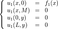
We divide this problem into 4 sub-problems, each one containing one of the non-homogeneous boundary conditions and each one subject to the Laplace equation condition,

We get the following boundary conditions for the 4 sub-problems:

In this case, we used all Dirichlet type boundary conditions, meaning that the boundary condition depends on the function value (e.g.

). If you are using any combination of Dirichlet, Neumann (e.g.

), Robin (e.g.

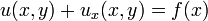
) types of boundary conditions, the types of the boundary conditions should be preserved in every sub-problem (e.g.
if

, then the boundary condition is

when the boundary condition is made homogeneous and

when it is the non-homogeneous boundary condition in a sub-problem).

Using the superposition principle, the complete solution to the 4 non-homogeneous boundary condition case is constructed by adding up all the solutions from the 4 sub-problems. In equation form,

Each sub-problem can be solved using the method for the case with 1 non-homogeneous boundary
condition as shown above.

Retrieved from "http://en.wikiversity.org/w/index.php?title=Laplace_Equation&oldid=665761"

Personal tools
Log in / create account

Namespaces
Resource

Discuss

Variants

Views
Read

Edit

View history

Actions

Search