An R Time Series Tutorial
2010-11-11 16:33
369 查看
An R Time Series Tutorial
Here are some examples that may help you become familiar with analyzing time series using R. You can copy-and-paste the R commands (multiple lines are ok) from this page into R. Printed output is blue. I suggest that you have R up and running before you start this tutorial.Please note that this is not a lesson in time series analysis. Also, the analyses performed on this page are simply demonstrations, they are not meant to be optimal or complete in any way. This is done intentionally so as not to spoil the fun you'll have working on the problems in the text.
If you're new to R/Splus, I suggest reading R for Beginners (a pdf file) first. Another good read for exploring time series isEconometrics in R (a pdf file). You may also want to poke around the QuickR website.
◊ Baby steps... your first R session. Get comfortable, then start her up and try some simple addition:
2+2
[1] 5
Ok, now you're an expert useR. It's time to move on to time series. What you'll see in the following examples should be enough to get you through the first four chapters of the text.
Let's play with the Johnson & Johnson data set. Download jj.dat to a directory called mydata (or wherever you choose ... the examples below and in the text assume the data are in that directory).
jj = scan("/mydata/jj.dat")        # read the data
jj <- scan("/mydata/jj.dat")       # read the data another way
scan("/mydata/jj.dat") -> jj       # and another
The R people (yes, they exist) prefer that you use the second [<-] or third [->] assignment operator, but your wrists and health care professionals prefer that you use the simpler first [=] method if you can.
Next, print jj (to the screen)
jj
[1]  0.71  0.63  0.85  0.44
[5]  0.61  0.69  0.92  0.55
.     .     .     .     .
.     .     .     .     .
[77] 14.04 12.96 14.85  9.99
[81] 16.20 14.67 16.02 11.61
and you see that jj is a collection of 84 numbers called an object. You can see all of your objects by typing
objects()
If you're a Matlab (or similar) user, you may think jj is an 84 × 1 vector, but it's not. It has order and length, but no dimensions (no rows, no columns). R call these objects vectors so you have to be careful. In R, matrices have dimensions but vectors do not. To wit:
jj[1]       # the first element
[1] 0.71
jj[84]      # the last element
[1] 11.61
jj[1:4]     # the first 4 elements
[1] 0.71 0.63 0.85 0.44
jj[-(1:80)] # everything EXCEPT the first 80 elements
[1] 16.20 14.67 16.02 11.61
length(jj)  # the number of elements
[1] 84
dim(jj)     # but no dimensions ...
NULL
nrow(jj)    # ... no rows
NULL
ncol(jj)    # ... and no columns
NULL
#-- if you want it to be a column vector (in R, a matrix), an easy way to go is:
jj = as.matrix(jj)
dim(jj)
[1] 84  1
Now, let's make jj a time series object.
jj = ts(jj, start=1960, frequency=4)
Note that the data are quarterly earnings, hence the frequency=4 statement. One nice thing about R is you can do a bunch of stuff (technical term) in one line. For example, you can read the data into jj and make it a time series object at the same time:
jj = ts(scan("/mydata/jj.dat"), start=1960, frequency=4)In the lines above, you can replace scan by read.table. Inputting data using read.table is an easy way to read a data file that is laid out as a matrix and may have headers (column descriptions). At this point, you might want to find out aboutread.table, data frames, and time series objects:
jj = ts(read.table("/mydata/jj.dat"), start=1960, frequency=4)
help(read.table)
help(ts)
help(data.frame)
There is a difference between scan and read.table. The former produces a vector (no dimensions) while the latter produces a data frame (and has dimensions).
One final note on reading the data. If the data started on the third quarter of 1960, say, then you would have something likets(x, start=c(1960,3), frequency=4) and so on. If you had monthly data that started from June, 1984, then you would havets(x, start=c(1984,6), frequency=12).
Let's view the data again as a time series object:
jj
Qtr1  Qtr2  Qtr3  Qtr4
1960  0.71  0.63  0.85  0.44
1961  0.61  0.69  0.92  0.55
.     .     .     .     .
.     .     .     .     .
1979 14.04 12.96 14.85  9.99
1980 16.20 14.67 16.02 11.61
Notice the difference? You also get some nice things with the ts object, for example, the corresponding time values:
time(jj)
Qtr1    Qtr2    Qtr3    Qtr4
1960 1960.00 1960.25 1960.50 1960.75
1961 1961.00 1961.25 1961.50 1961.75
.     .     .     .     .     .
.     .     .     .     .     .
1979 1979.00 1979.25 1979.50 1979.75
1980 1980.00 1980.25 1980.50 1980.75
By the way, you could have put the data into jj and printed it at the same time by enclosing the command:
(jj = ts(scan("/mydata/jj.dat"), start=1960, frequency=4))Now try a plot of the data:
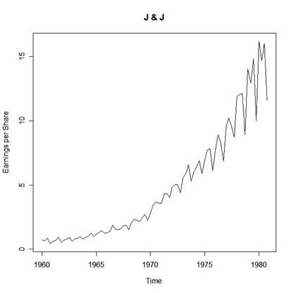
plot(jj, ylab="Earnings per Share", main="J & J")
with the result being:
 |
plot(jj, type="o", col="blue", lty="dashed")
plot(diff(log(jj)), main="logged and diffed")
and while you're here, check out plot.ts and ts.plot:
x = -5:5                  # sequence of integers from -5 to 5
y = 5*cos(x)              # guess
par(mfrow=c(3,2))         # multifigure setup: 3 rows, 2 cols
#---  plot:
plot(x, main="plot(x)")
plot(x, y, main="plot(x,y)")
#---  plot.ts:
plot.ts(x, main="plot.ts(x)")
plot.ts(x, y, main="plot.ts(x,y)")
#---  ts.plot:
ts.plot(x, main="ts.plot(x)")
ts.plot(ts(x), ts(y), col=1:2, main="ts.plot(x,y)")  # note- x and y are ts objects
#---  the help files [? and help() are the same]:
?plot.ts
help(ts.plot)
?par        # might as well skim the graphical parameters help file while you're here
 |
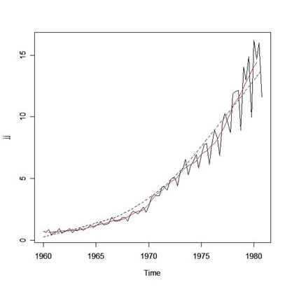
How about filtering/smoothing the Johnson & Johnson series using a two-sided moving average? Let's try this:
fjj(t) = ⅛ jj(t-2) + ¼ jj(t-1) + ¼ jj(t) + ¼ jj(t+1) + ⅛ jj(t+2)
and we'll add a lowess fit for fun.
k = c(.5,1,1,1,.5)            # k is the vector of weights
(k = k/sum(k))
[1] 0.125 0.250 0.250 0.250 0.125
fjj = filter(jj, sides=2, k)  # ?filter for help [but you knew that already]
plot(jj)
lines(fjj, col="red")         # adds a line to the existing plot
lines(lowess(jj), col="blue", lty="dashed")
... and the result:
 |
dljj = diff(log(jj))        # difference the logged data
plot(dljj)                  # plot it if you haven't already
shapiro.test(dljj)          # test for normality
Shapiro-Wilk normality test
data:  dljj
W = 0.9725, p-value = 0.07211
Now a histogram and a Q-Q plot, one on top of the other:
par(mfrow=c(2,1))        # set up the graphics
hist(dljj, prob=TRUE, 12)   # histogram
lines(density(dljj))     # smooth it - ?density for details
qqnorm(dljj)             # normal Q-Q plot
qqline(dljj)             # add a line
and the results:
 |
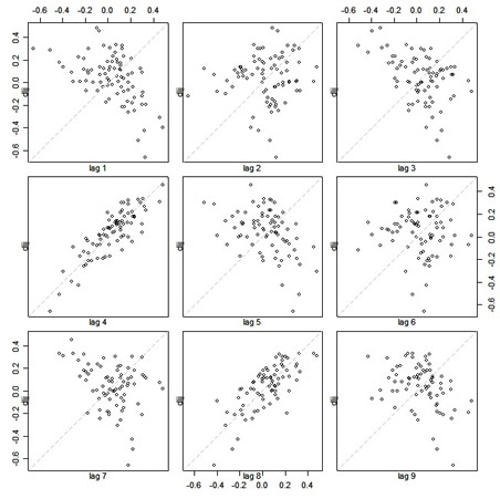
lag.plot(dljj, 9, do.lines=FALSE) # why the do.lines=FALSE? ... try leaving it out
Notice the large positive correlation at lags 4 and 8 and the negative correlations at a few other lags:
 |
par(mfrow=c(2,1)) # The power of accurate observation is commonly called cynicism
#     by those who have not got it. - George Bernard Shaw
acf(dljj, 20)     # ACF to lag 20 - no graph shown... keep reading
pacf(dljj, 20)    # PACF to lag 20 - no graph shown... keep reading
# !!NOTE!! acf2 on the line below is NOT available in R... details follow the graph below
acf2(dljj)        # this is what you'll see below
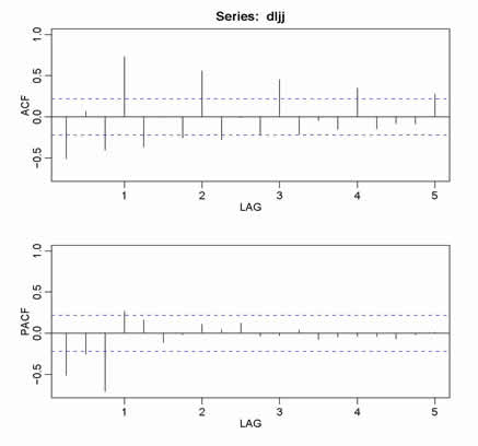 |
◊ Ok- here's the story on acf2. I like my ACF and PACF a certain way, which is not the default R way. So, I wrote a little script called acf2.R that you can read about and obtain here: Examples (there are other goodies there).
Moving on, let's try a structural decomposition of log(jj) = trend + season + error using lowess. Note, this example works only if jj is dimensionless (i.e., you didn't read it in using read.table ... thanks to Jon Moore of the University of Reading, U.K., for pointing this out.)
plot(dog <- stl(log(jj), "per"))
Here's what you get:
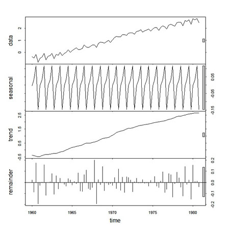 |
◊ This is a good time to explain $. In the above, dog is an object containing a bunch of things (technical term). If you type dog, you'll see the components, and if you type summary(dog) you'll get a little summary of the results. One of the components ofdog is time.series, which contains the resulting series (seasonal, trend, remainder). To see this component of the object dog, you type dog$time.series (and you'll see 3 series, the last of which contains the residuals). And that's the story of $ ... you'll see more examples as we move along.
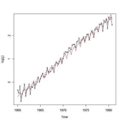
And now, we'll do some of Problem 2.1. We're going to fit the regression
log(jj)= β*time + α1*Q1 + α2*Q2 + α3*Q3 + α4*Q4 + ε
where Qi is an indicator of the quarter i = 1,2,3,4. Then we'll inspect the residuals.
Q = factor(rep(1:4,21))     # make (Q)uarter factors [that's repeat 1,2,3,4, 21 times]
trend = time(jj)-1970   # not necessary to "center" time, but the results look nicer
reg = lm(log(jj)~0+trend+Q, na.action=NULL)  # run the regression without an intercept
#-- the na.action statement is to retain time series attributes
summary(reg)
Call:
lm(formula = log(jj) ~ 0 + trend + Q, na.action = NULL)

Residuals:
Min       1Q   Median       3Q      Max
-0.29318 -0.09062 -0.01180  0.08460  0.27644

Coefficients:
Estimate Std. Error t value Pr(>|t|)
trend 0.167172   0.002259   74.00   <2e-16 ***
Q1    1.052793   0.027359   38.48   <2e-16 ***
Q2    1.080916   0.027365   39.50   <2e-16 ***
Q3    1.151024   0.027383   42.03   <2e-16 ***
Q4    0.882266   0.027412   32.19   <2e-16 ***
---
Signif. codes:  0 '***' 0.001 '**' 0.01 '*' 0.05 '.' 0.1 ' ' 1

Residual standard error: 0.1254 on 79 degrees of freedom
Multiple R-squared: 0.9935,     Adjusted R-squared: 0.9931
F-statistic:  2407 on 5 and 79 DF,  p-value: < 2.2e-16
You can view the model matrix (with the dummy variables) this way:
model.matrix(reg)

trend Q1 Q2 Q3 Q4   (remember trend is time centered at 1970)
1  -10.00  1  0  0  0
2   -9.75  0  1  0  0
3   -9.50  0  0  1  0
4   -9.25  0  0  0  1
5   -9.00  1  0  0  0
6   -8.75  0  1  0  0
7   -8.50  0  0  1  0
8   -8.25  0  0  0  1
.     .    .  .  .  .
.     .    .  .  .  .
81  10.00  1  0  0  0
82  10.25  0  1  0  0
83  10.50  0  0  1  0
84  10.75  0  0  0  1
Now check out what happened. Look at a plot of the observations and their fitted values:
plot(log(jj), type="o")   # the data in black with little dots
lines(fitted(reg), col=2) # the fitted values in bloody red - or use lines(reg$fitted, col=2)
you get:
 |
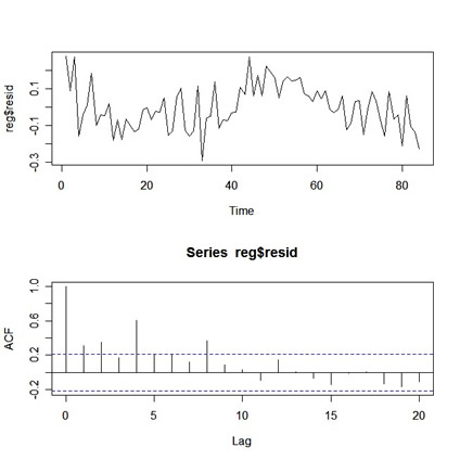
par(mfrow=c(2,1))
plot(resid(reg))      # residuals - reg$resid is same as resid(reg)
acf(resid(reg),20)    # acf of the resids
and you get:
 |
You have to be careful when you regress one time series on lagged components of another using lm(). There is a package called dynlm that makes it easy to fit lagged regressions, and I'll discuss that right after this example. If you use lm(), then what you have to do is "tie" the series together using ts.intersect. If you don't tie the series together, they won't be aligned properly. Here's an example regressing weekly cardiovascular mortality (cmort.dat) on particulate pollution (part.dat) at the present value and lagged four weeks (about a month). For details about the data set, see Chapter 2.
mort = ts(scan("/mydata/cmort.dat"),start=1970, frequency=52)  # make these time series objects
Read 508 items
part = ts(scan("/mydata/part.dat"),start=1970, frequency=52)
Read 508 items
ded = ts.intersect(mort,part,part4=lag(part,-4), dframe=TRUE) # tie them together in a data frame
fit = lm(mort~part+part4, data=ded, na.action=NULL)         # now the regression will work
summary(fit)
Call:
lm(formula = mort ~ part + part4, data = ded, na.action = NULL)

Residuals:
Min       1Q   Median       3Q      Max
-22.7429  -5.3677  -0.4136   5.2694  37.8539

Coefficients:
Estimate Std. Error t value Pr(>|t|)
(Intercept) 69.01020    1.37498  50.190  < 2e-16 ***
part         0.15140    0.02898   5.225 2.56e-07 ***
part4        0.26297    0.02899   9.071  < 2e-16 ***
---
Signif. codes:  0 '***' 0.001 '**' 0.01 '*' 0.05 '.' 0.1 ' ' 1

Residual standard error: 8.323 on 501 degrees of freedom
Multiple R-Squared: 0.3091,     Adjusted R-squared: 0.3063
F-statistic: 112.1 on 2 and 501 DF,  p-value: < 2.2e-16
Note: There was no need to rename lag(part,-4) to part4, it's just an example of what you can do.
An alternative to the above is the package dynlm, which has to be installed [for details, in R type help(INSTALL) orhelp("install.packages") ]. After the package is installed, you can do the previous example as follows:
library(dynlm)                         # load the package
fit = dynlm(mort~part + lag(part,-4))  # assumes mort and part are ts objects
# fit = dynlm(mort~part + L(part,4))  is the same thing.
summary(fit)
Call:
dynlm(formula = mort ~ part + lag(part, -4))

Residuals:
Min       1Q   Median       3Q      Max
-22.7429  -5.3677  -0.4136   5.2694  37.8539

Coefficients:
Estimate Std. Error t value Pr(>|t|)
(Intercept)   69.01020    1.37498  50.190  < 2e-16 ***
part           0.15140    0.02898   5.225 2.56e-07 ***
lag(part, -4)  0.26297    0.02899   9.071  < 2e-16 ***
---
Signif. codes:  0 '***' 0.001 '**' 0.01 '*' 0.05 '.' 0.1 ' ' 1

Residual standard error: 8.323 on 501 degrees of freedom
Multiple R-Squared: 0.3091,     Adjusted R-squared: 0.3063
F-statistic: 112.1 on 2 and 501 DF,  p-value: < 2.2e-16
Well, it's time to simulate. The workhorse for ARIMA simulations is arima.sim(). Here are some examples; no output is shown here so you're on your own.
# some AR1s
x1 = arima.sim(list(order=c(1,0,0), ar=.9), n=100)
x2 = arima.sim(list(order=c(1,0,0), ar=-.9), n=100)
par(mfrow=c(2,1))
plot(x1, main=(expression(AR(1)~~~phi==+.9)))      # ~ is a space and == is equal
plot(x2, main=(expression(AR(1)~~~phi==-.9)))
x11()                                         # open another graphics device if you wish
par(mfcol=c(2,2))
acf(x1, 20)
acf(x2, 20)
pacf(x1, 20)
pacf(x2, 20)
# you could have, for example, used acf2(x1)
# to get the ACF and PACF of x1 (or x2)... if you had acf2.R, of course.

# an MA1
x = arima.sim(list(order=c(0,0,1), ma=.8), n=100)
par(mfcol=c(3,1))
plot(x, main=(expression(MA(1)~~~theta==.8)))
acf(x,20)
pacf(x,20)

# an AR2
x = arima.sim(list(order=c(2,0,0), ar=c(1,-.9)), n=100)
par(mfcol=c(3,1))
plot(x, main=(expression(AR(2)~~~phi[1]==1~~~phi[2]==-.9)))
acf(x, 20)
pacf(x, 20)

# an ARIMA(1,1,1)
x = arima.sim(list(order=c(1,1,1), ar=.9, ma=-.5), n=200)
par(mfcol=c(3,1))
plot(x, main=(expression(ARIMA(1,1,1)~~~phi==.9~~~theta==-.5)))
acf(x, 30)  # the process is not stationary, so there is no population [P]ACF ...
pacf(x, 30) # but look at the sample values to see how they differ from the examples above
◊ Next, we're going to do some ARIMA estimation. This gets a bit tricky because R is not useR friendly when it comes to fitting ARIMA models. Much of the story is spelled out in our R Issues page. I'll be as gentle as I can at first.
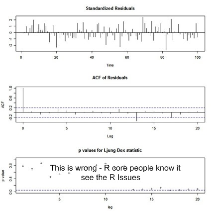
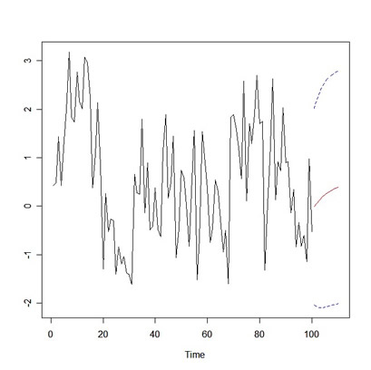
First, we'll fit an ARMA model to some simulated data (with diagnostics and forecasting):
x = arima.sim(list(order=c(1,0,1), ar=.9, ma=-.5), n=100) # simulate some data
(x.fit = arima(x, order = c(1, 0, 1)))   # fit the model and print the results

Call: arima(x = x, order = c(1, 0, 1))
Coefficients:
ar1      ma1  intercept <-- NOT the intercept - see R Issue 1
0.8465  -0.5021     0.5006
s.e.  0.0837   0.1356     0.3150
sigma^2 estimated as 1.027:  log likelihood = -143.44,  aic = 294.89
... diagnostics:
tsdiag(x.fit, gof.lag=20) # you know the routine- ?tsdiag for details
... and the output
 |
x.fore = predict(x.fit, n.ahead=10)
# plot the forecasts
U = x.fore$pred + 2*x.fore$se
L = x.fore$pred - 2*x.fore$se
minx=min(x,L)
maxx=max(x,U)
ts.plot(x,x.fore$pred,col=1:2, ylim=c(minx,maxx))
lines(U, col="blue", lty="dashed")
lines(L, col="blue", lty="dashed")
... and here's the plot of the data and the forecasts (with error bounds):
 |
u = read.table("/mydata/globtemp2.dat")    # read the data
gtemp = ts(u[,2], start=1880, freq=1)      # yearly temp in col 2
plot(gtemp)                                # graph the series (not shown here)
... long story short, the data appear to be an ARIMA(1,1,1) with a drift of about +.6 oC per century (and hence the global warming hypothesis). Let's fit the model:
arima(gtemp, order=c(1,1,1))
Coefficients:
ar1      ma1
0.2545  -0.7742
s.e.  0.1141   0.0651
So what's wrong? .... well, there's no estimate of the drift!! With no drift, the global warming hypothesis is kaput (technical term)... that is, the temps are just basically taking a random walk. How do you get the estimate of drift?... do this:
arima(diff(gtemp), order=c(1,0,1))  # diff the data and fit an arma to the diffed data
Coefficients:
ar1      ma1  intercept
0.2695  -0.8180     0.0061
s.e.  0.1122   0.0624     0.0030
What happened? The two runs should have given the same results, but the default models for the two cases are different. I won't go into detail here because the details can be found on the R Issues page. And, of course, this problem continues if you try to do forecasting. There are remedies. One remedy is to do the following:
drift = 1:length(gtemp)
arima(gtemp, order=c(1,1,1), xreg=drift)
Coefficients:
ar1      ma1   drift
0.2695  -0.8180  0.0061
s.e.  0.1122   0.0624  0.0030
and then make sure you continue the along these lines when you forecast. Another remedy is to use the scripts calledsarima.R for model fitting, and sarima.for.R for forecasting. You can get those scripts with some details on this page:Examples.
◊ You may not have understood all the details of this example, but at least you should realize that you may get into trouble when fitting ARIMA models with R. In particular, you should come away from this realizing that, in R, arima(x, order=c(1,1,1))is different than arima(diff(x), order=c(1,0,1)) and arima calls the estimate of the mean the intercept. Again, much of the story is spelled out in our R Issues page.
And now for some regression with autocorrelated errors. This can be accomplished two different ways. First, we'll usegls() from the package nlme, which you have to load. We're going to fit the model Mt = α + βt + γPt + et where Mt and Pt are the mortality and particulates series from a previous example, and et is autocorrelated error.
library(nlme)            # load the package
trend = time(mort)       # assumes mort and part are there from previous examples
fit.lm = lm(mort~trend + part)  # ols
acf(resid(fit.lm))       # check acf and pacf of the resids
pacf(resid(fit.lm))      # or use acf2(resid(fit.lm)) if you have acf2
# resids appear to be AR(2) ... now use gls() from nlme:
fit.gls = gls(mort~trend + part, correlation=corARMA(p=2), method="ML")
# take 5 ........................................
#................................................
#................................................
#................................................
# done:
summary(fit.gls)
Parameter estimate(s):
Phi1      Phi2
0.3980566 0.4134305
Coefficients:     Value  Std.Error   t-value  p-value
(Intercept)   3131.5452   857.2141  3.653166    3e-04
trend           -1.5444     0.4340 -3.558021    4e-04
part             0.1503     0.0210  7.162408    0e+00

# resid analysis- we assumed et = φ1 et-1 + φ2 et-2 + wt where wt is white.
w = filter(resid(fit.gls), filter=c(1,-.3980566, -.4134305), sides=1)  # get resids
w = w[-2:-1]                   # first two are NA
Box.test(w, 12, type="Ljung")  # check whiteness via Ljung-Box-Pierce statistic
X-squared = 8.6074, df = 12, p-value = 0.736
pchisq(8.6074, 10, lower=FALSE)    # the p-value (they are resids from an ar2 fit)
[1] 0.569723
Now, we'll doing the same thing using arima(), which is easier and a little quicker.
(fit2.gls = arima(mort, order=c(2,0,0), xreg=cbind(trend, part)))
Coefficients:
ar1     ar2  intercept    trend    part
0.3980  0.4135  3132.7085  -1.5449  0.1503
s.e.  0.0405  0.0404   854.6662   0.4328  0.0211
sigma^2 estimated as 28.99:  log likelihood = -1576.56,  aic = 3165.13

Box.test(resid(fit2.gls), 12, type="Ljung")   # and so on ...
◊ ARMAX: If you want to fit an ARMAX model you have to do it via a state space model... more details will follow on the Chapter 6 page when I have the time. As seen above, using xreg in arima() does NOT fit an ARMAX model, which is too bad, but the help file (?arima) didn't say it did. For more info, head on over to the R Issues page and check out Issue 2.
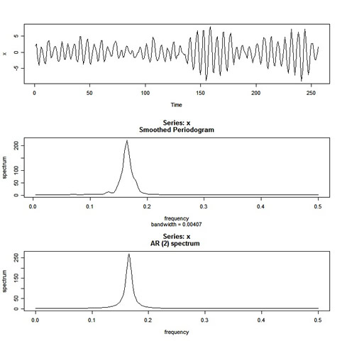
Finally, a spectral analysis quicky:
x = arima.sim(list(order=c(2,0,0), ar=c(1,-.9)), n=2^8) # some data
(u = polyroot(c(1,-1,.9)))            # x is AR(2) w/complex roots
[1] 0.5555556+0.8958064i 0.5555556-0.8958064i
Arg(u[1])/(2*pi)                      # dominant frequency around .16:
[1] 0.1616497
par(mfcol=c(3,1))
plot.ts(x)
spec.pgram(x, spans=c(3,3), log="no")  # nonparametric spectral estimate; also see spectrum()
?spec.pgram                            # some help
'spec.pgram' calculates the periodogram using a fast Fourier
transform, and optionally smooths the result with a series of
modified Daniell smoothers (moving averages giving half weight to
the end values).
spec.ar(x, log="no")                   # parametric spectral estimate
and the graph:
 |
(转自:http://www.stat.pitt.edu/stoffer/tsa2/R_time_series_quick_fix.htm)

相关文章推荐
- An R Time Series Tutorial
- How to Save an ARIMA Time Series Forecasting Model in Python (如何在Python中保存ARIMA时间序列预测模型)
- 数据挖掘中的时序数据分析方法(According to Eamonn Keogh’s Time Series Tutorial)
- DCM TUTORIAL – AN INTRODUCTION TO ORIENTATION KINEMATICS (REV 0.1)
- The Python Tutorial 3——An Informal Introduction to Python
- Alternativa 3D Series – Tutorial 1 – Getting Started
- A time series contest attempt
- libsqlora8:(insert system time as an appointed format)
- An ffmpeg and SDL Tutorial
- An Implemention of Realtime Gobal Illumination
- Becoming an Xperf Xpert Part 6: RIP Xperf. Time to Learn Windows Performance Analyzer!
- 【译】TetroGL: An OpenGL Game Tutorial in C++ for Win32 Platforms - Part 2 (上)
- 关于Quartus编译的问题:Error:Can't generate netlist outout files because the file"C:/altera/ XXXXXXXX" is an OpenCore Plus time-limited file.
- iOS: How do you measure actual on-CPU time for an iOS thread?
- bug宝典 hadoop篇 /hadoop/hdfs/data is in an inconsistent state: file VERSION has cTime missing.
- An AODV Tutorial
- JWT Authentication Tutorial: An example using Spring Boot--转
- Tutorial: Schedule an XS Job
- Give an O(lg n)-time algorithm to find the median of all 2n elements in arrays X and Y.
- An ffmpeg and SDL Tutorial 01