The Predator-Prey Equation in Matlab
2010-07-31 15:43
288 查看
转载自:http://www-users.math.umd.edu/~jmr/246/predprey.html
Critical points:
Phase Plot
Plot of Populations vs. Time
Modified Model with "Limits to Growth" for Prey (in Absence of Predators)
Critical points:
Plot of Populations vs. Time
Original Lotka-Volterra Model
We assume we have two species, herbivores with population x,
and predators with propulation y. We assume that x grows exponentially
in the absence of predators, and that y decays exponentially in
the absence of prey. Consider, say, the system

Critical points:
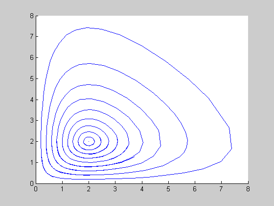
Thus we have a center at (2, 2) and a saddle point at (0, 0), at least for the linearized system. This suggests the possibility
of periodic orbits centered around (2, 2).
Phase Plot
Plot of Populations vs. Time
We color-code the plots so you can see which ones go together.
Modified Model with "Limits to Growth" for Prey (in Absence of Predators)
In the original equation, the population of prey increases indefinitely in the absence of predators. This is unrealistic,
since they will eventually run out of food, so let's add another term limiting growth and change the system to

Critical points:
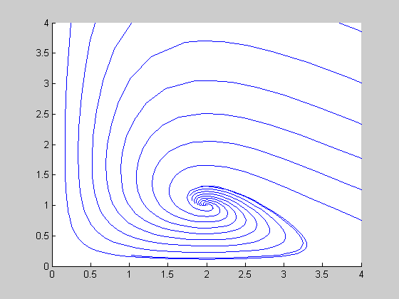
Thus we have saddles at (0, 0), (4, 0) and a stable spiral point at (2, 1).
Plot of Populations vs. Time
Published with MATLAB® 7.0
The Predator-Prey Equation
Contents
Original Lotka-Volterra ModelCritical points:
Phase Plot
Plot of Populations vs. Time
Modified Model with "Limits to Growth" for Prey (in Absence of Predators)
Critical points:
Plot of Populations vs. Time
Original Lotka-Volterra Model
We assume we have two species, herbivores with population x, and predators with propulation y. We assume that x grows exponentially
in the absence of predators, and that y decays exponentially in
the absence of prey. Consider, say, the system
Critical points:
syms x
 y

vars = [x, y];
eqs = [x*(1-y/2), y*(-1+x/2)];
[xc, yc] = solve(eqs(1), eqs(2));
[xc, yc]
A = jacobian(eqs, vars);
disp('Matrix of linearized system:'
)
subs(A, vars, [xc(1), yc(1)])
disp('eigenvalues:'
)
eig(ans)
disp('Matrix of linearized system:'
)
subs(A, vars, [xc(2), yc(2)])
disp('eigenvalues:'
)
eig(double(ans))
ans =
[ 0, 0]
[ 2, 2]
Matrix of linearized system:
ans =
[ 1, 0]
[ 0, -1]
eigenvalues:
ans =
1
-1
Matrix of linearized system:
ans =
[ 0, -1]
[ 1, 0]
eigenvalues:
ans =
0 + 1.0000i
0 - 1.0000iThus we have a center at (2, 2) and a saddle point at (0, 0), at least for the linearized system. This suggests the possibility
of periodic orbits centered around (2, 2).
Phase Plot
rhs1 = @(t, x) ...
[x(1)*(1-.5*x(2)); x(2)*(-1+.5*x(1))];
options = odeset('RelTol'
, 1e-6);
figure, hold on
for
x0 = 0:.2:2
[t, x] = ode45(rhs1, [0, 10], [x0;2]);
plot(x(:,1), x(:,2))
end
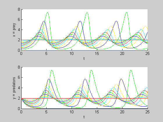
, hold offPlot of Populations vs. Time
We color-code the plots so you can see which ones go together.colors = 'rgbyc'
;
figure, hold on
for
x0 = 0:10
[t, x] = ode45(rhs1, [0, 25], [x0/5; 2], options);
subplot(2, 1, 1), hold on
plot(t, x(:,1), colors(mod(x0,5)+1))
subplot(2, 1, 2), hold on
plot(t, x(:, 2), colors(mod(x0,5)+1))
hold on
end
subplot(2, 1, 1)
xlabel t
ylabel 'x = prey'
subplot(2, 1, 2)
xlabel t
ylabel 'y = predators'
hold offModified Model with "Limits to Growth" for Prey (in Absence of Predators)
In the original equation, the population of prey increases indefinitely in the absence of predators. This is unrealistic,since they will eventually run out of food, so let's add another term limiting growth and change the system to
Critical points:
syms x
 y

vars = [x, y];
eqs = [x*(1-y/2-x/4), y*(-1+x/2)];
[xc, yc] = solve(eqs(1), eqs(2));
[xc, yc]
A = jacobian(eqs, vars);
disp('Matrix of linearized system:'
)
subs(A, vars, [xc(1), yc(1)])
disp('eigenvalues:'
)
eig(ans)
disp('Matrix of linearized system:'
)
subs(A, vars, [xc(2), yc(2)])
disp('eigenvalues:'
)
eig(ans)
disp('Matrix of linearized system:'
)
subs(A, vars, [xc(3), yc(3)])
disp('eigenvalues:'
)
eig(double(ans))
ans = [ 0, 0] [ 4, 0] [ 2, 1] Matrix of linearized system: ans = [ 1, 0] [ 0, -1] eigenvalues: ans = 1 -1 Matrix of linearized system: ans = [ -1, -2] [ 0, 1] eigenvalues: ans = -1 1 Matrix of linearized system: ans = [ -1/2, -1] [ 1/2, 0] eigenvalues: ans = -0.2500 + 0.6614i -0.2500 - 0.6614i
Thus we have saddles at (0, 0), (4, 0) and a stable spiral point at (2, 1).
rhs2 = @(t, x) ...

    [x(1)*(1-.5*x(2)-0.25*x(1)); x(2)*(-1+.5*x(1))];
figure, hold on

for
 x0 = 0:.2:2
    [t, x] = ode45(rhs2, [0, 10], [x0;1]);
    plot(x(:,1), x(:,2))
end

for
 x0 = 0:.2:2
    [t, x] = ode45(rhs2, [0, -10], [x0;1]);
    plot(x(:,1), x(:,2))
end

axis([0, 4, 0, 4]), hold off
Warning: Failure at t=-3.380660e+000. Unable to meet integration tolerances without reducing the step size below the smallest value allowed (7.105427e-015) at time t. Warning: Failure at t=-3.535072e+000. Unable to meet integration tolerances without reducing the step size below the smallest value allowed (7.105427e-015) at time t. Warning: Failure at t=-3.735844e+000. Unable to meet integration tolerances without reducing the step size below the smallest value allowed (7.105427e-015) at time t. Warning: Failure at t=-3.984664e+000. Unable to meet integration tolerances without reducing the step size below the smallest value allowed (7.105427e-015) at time t. Warning: Failure at t=-4.299922e+000. Unable to meet integration tolerances without reducing the step size below the smallest value allowed (1.421085e-014) at time t. Warning: Failure at t=-4.719481e+000. Unable to meet integration tolerances without reducing the step size below the smallest value allowed (1.421085e-014) at time t. Warning: Failure at t=-5.332082e+000. Unable to meet integration tolerances without reducing the step size below the smallest value allowed (1.421085e-014) at time t. Warning: Failure at t=-6.437607e+000. Unable to meet integration tolerances without reducing the step size below the smallest value allowed (1.421085e-014) at time t.
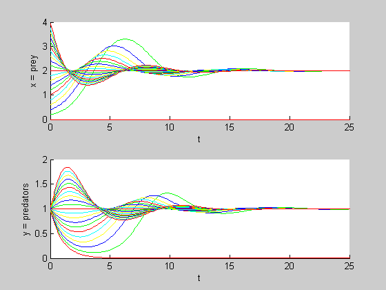
Plot of Populations vs. Time
figure, hold on

for
 x0 = 0:20
    [t, x] = ode45(rhs2, [0, 25], [x0/5; 1], options);
    subplot(2, 1, 1), hold on

    plot(t, x(:,1), colors(mod(x0,5)+1))
    subplot(2, 1, 2), hold on

    plot(t, x(:, 2), colors(mod(x0,5)+1))
    hold on

end

subplot(2, 1, 1)
xlabel t

ylabel 'x = prey'

subplot(2, 1, 2)
xlabel t

ylabel 'y = predators'

hold off
Published with MATLAB® 7.0

相关文章推荐
- 数字图像处理实验(9):PROJECT 04-05,Correlation in the Frequency Domain 标签: 图像处理MATLAB 2017-05-25 10:14
- GPU Programming in MATLAB
- matlab 标定箱错误:Disabling view 2 - Reason: the left and right images are found inconsistent (已解决)
- pickle file in matlab
- How can I plot an image (.jpg) in MATLAB in both 2-D and 3-D?
- matlab kmeans :failed to converge in 100 iterations
- Specify Callbacks in Function Calls matlab
- itk vtk in matlab
- Use matlab to traverse the files in a folder
- 1 assert/signal failures have occurred; MATLAB will abort in 10 seconds
- add a new path to visit in matlab
- Install Matlab in Ubuntu 12.04
- matlab inpolygon 判断点在多边形内
- Retinex in Matlab
- matllab shadows it in the matlab path
- Curve fitting in Matlab
- Matlab中显示法线方向 display normal map in matlab
- some encountered problem and the solve methods when install Matlab in Linux
- map() in matlab
- 课程: Introduction to Programming with MATLAB in coursera